Market Trend Analysis: Algorithmic Support and Resistance Detection
Tip: You can view and explore the original interactive Jupyter Notebook for this research paper on Kaggle.

Introduction
I have long been interested in financial markets. Over the years, I developed a trading strategy that generates modest profits. However, I often find myself manually handling various scenarios and constantly monitoring market quotes. Since I am both studying and working, my time is extremely limited, and I lack consistency in this field. As a result, I want to analyze my strategy in greater depth.
For this research, I have chosen to focus on the cryptocurrency market.
The research will center on the BTCUSDT trading pair, as it is the most popular instrument and its historical data is freely available on any cryptocurrency exchange. Additionally, BTCUSDT does not have premarket or postmarket trading, simplifying the analysis process.
The primary research question addressed in this project is: How effectively can support and resistance levels be identified using algorithmic methods? The objective: are to:
- Analyze patterns in cryptocurrency market movements.
- Develop and evaluate algorithms for constructing support and resistance levels.
- Investigate the applicability of these techniques to real-time trading scenarios.
Strategy Description: : Based on my observations, financial markets move in three major waves (sizes). These movements occur both in upward (Long) and downward (Short) directions. To identify these movements, it is crucial to establish support and resistance levels.
Support and resistance levels
Support and resistance levels are key concepts in technical analysis, aiding traders and investors in making informed decisions about buying or selling assets. These levels indicate price points where an asset encounters difficulty moving upward or downward.
Support level
A support level is a price point below which an asset struggles to fall. At this level, demand exceeds supply, preventing further price drops and potentially causing a reversal upward. Buyers perceive this price as attractive, believing the asset to be undervalued, and their increased activity halts the decline.
When an asset’s price reaches the support level, it often rebounds because investors consider this a favorable buying opportunity. The support level acts as a “cushion,” protecting the price from falling further.
Resistance level
A resistance level is a price point above which an asset struggles to rise. At this level, supply exceeds demand, halting price increases and potentially causing a reversal downward. Sellers see this price as overvalued and start selling, impeding further growth.
When an asset’s price reaches the resistance level, it frequently declines, as investors see this as an ideal selling opportunity. The resistance level serves as a “ceiling,” making it difficult for the price to break through.
Practical example
Let’s consider a simple example. Suppose a company’s stock has repeatedly risen to $50 over recent months but always retreated afterward. This price point becomes a resistance level. If the stock price breaks above this level and holds, it may signal the beginning of an uptrend.
Conversely, if the stock has repeatedly fallen to $45 but recovered each time, this becomes a support level. If the stock price falls below this level and holds, it may indicate the start of a downtrend.
References supporting definitions of support and resistance
BTCUSDT Example
To analyze, we’ll use the TradingView platform.
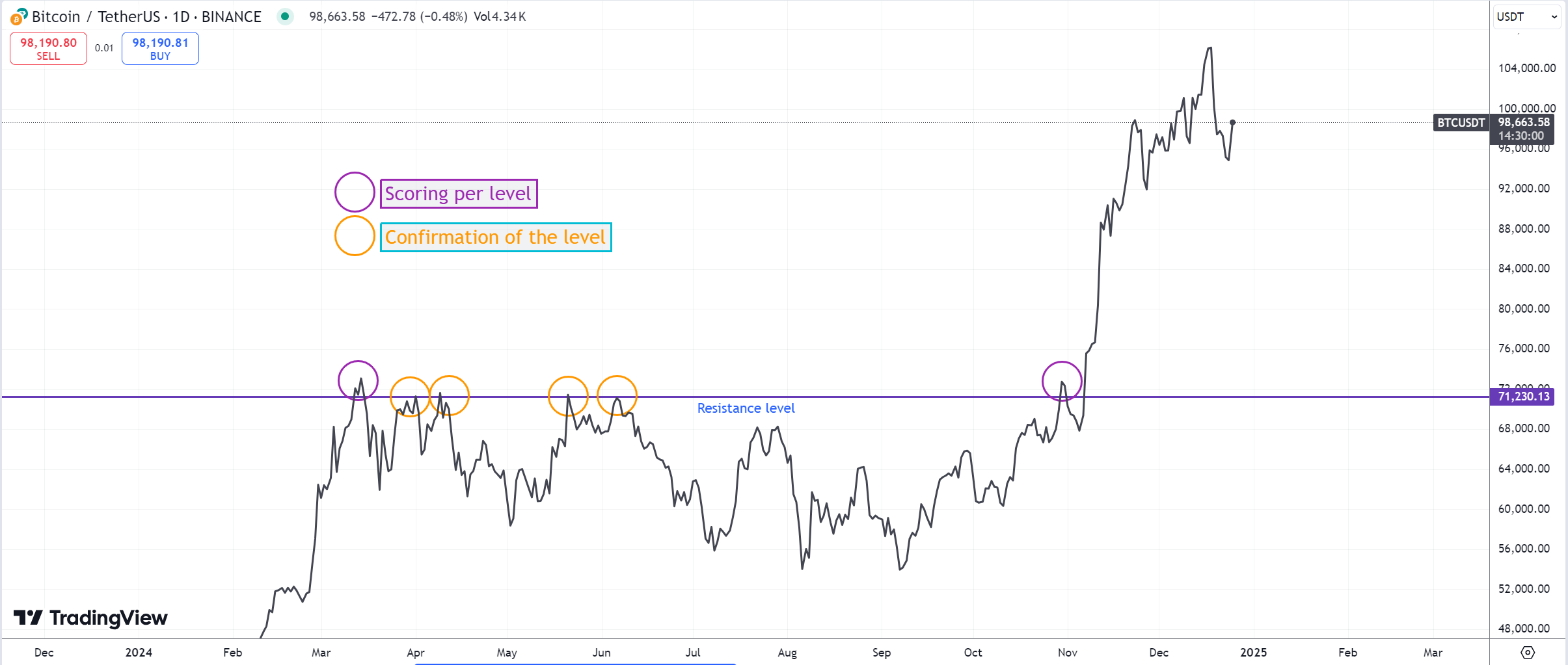
Why this is a resistance level: Multiple price touches confirm that this level is significant to market participants. Eventually, the level is broken with a liquidity sweep.
Expected results
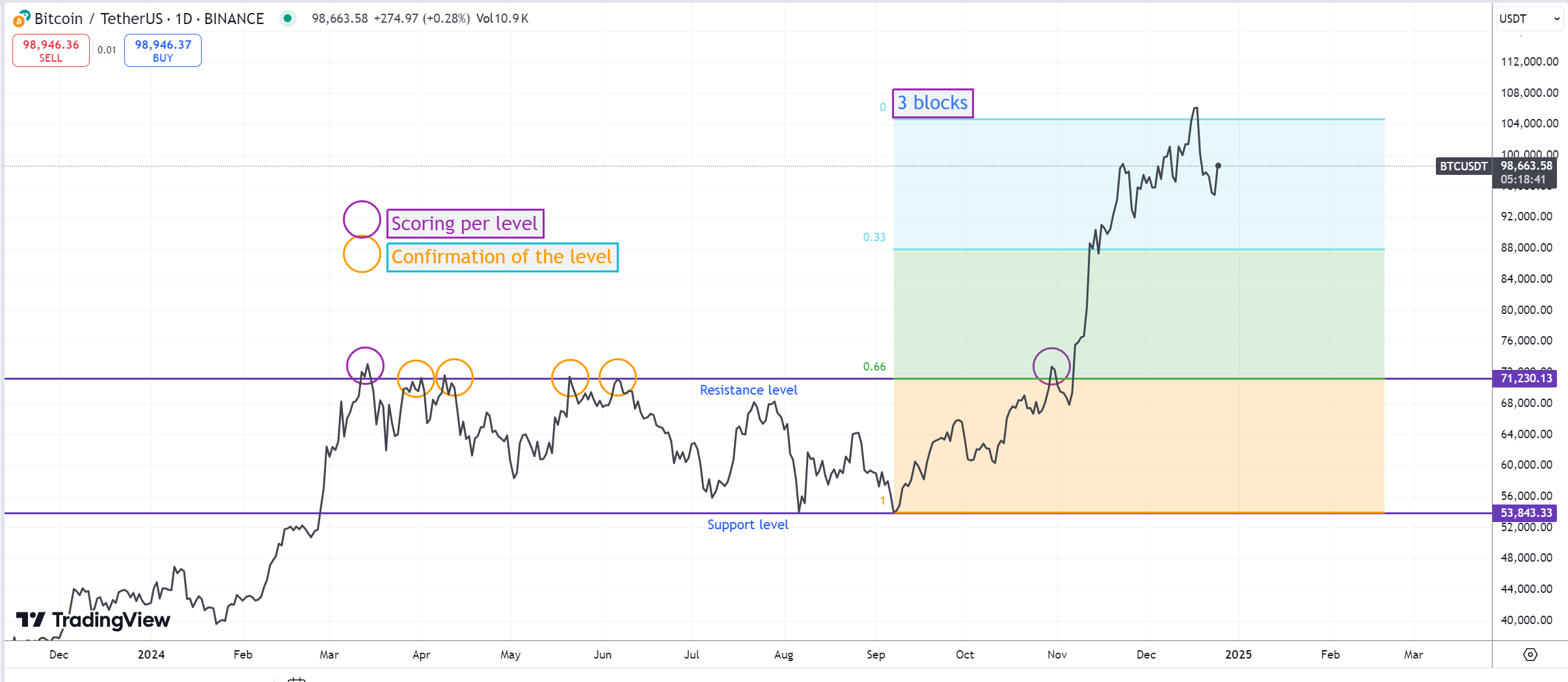
The market always moves in three blocks or waves (referred to hereafter as blocks), either up or down. It is essential to learn how to identify these correctly. This is challenging but these “three blocks” always align clearly with key levels. If the blocks fail to align with the levels, the chosen market volatility might be unsuitable.
Market volatility measures how frequently and sharply financial asset prices change over time. It reflects the market’s instability.
Another example with TONUSDT:
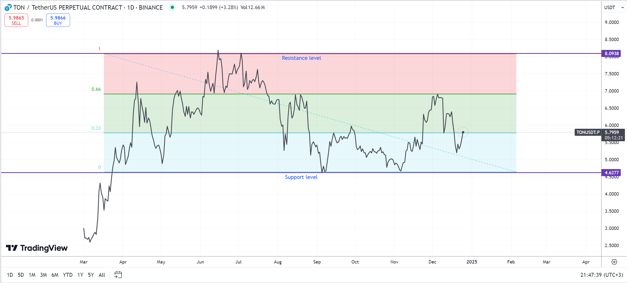
This is hard to visualize without extensive experience observing market behavior and charts.
Search for existing solutions
I explored various online sources but found no suitable method for identifying levels. One interesting resource is this Google Colab notebook I prefer constructing levels based on candle closures, unlike most methods that rely on candle wicks. This approach avoids distortions in analyzing price movement. My constructed objects on charts align closely with price movements, and the levels also appear accurate.
Why use chart analysis Instead of news analysis?
This work adopts technical analysis based on graphical data representation as the preferred approach due to the following reasons:
- Objectivity: Technical analysis uses objective data and statistical models, reducing subjective interpretations and biases.
- Predictability: It allows forecasting future trends based on historical data, especially valuable in volatile cryptocurrency markets.
- Analytical depth: Charts and indicators provide a more comprehensive understanding of market conditions and potential directions.
- Systematic approach: Technical analysis algorithms can be applied consistently and automated, increasing accuracy and reducing human error.
- Speed of changes: High cryptocurrency market volatility demands rapid response, challenging with news-based approaches.
- Risk management: Technical indicators help assess and manage risks, minimizing losses and protecting capital.
Ethics of data usage
The data used in this project is publicly available and anonymized, ensuring compliance with ethical guidelines. No personally identifiable information is included. Potential biases in the data, such as time-of-day effects or trading volume imbalances, have been noted and mitigated where possible. These methods and findings are intended solely for educational purposes.
Project execution plan
- Obtain publicly available data:
- Locate and download necessary data from exchange platforms or public sources.
- Data import and preparation in Jupyter Notebook:
- Import the data into Jupyter Notebook.
- Clean and preprocess the data for analysis.
- Develop methods for identifying support and resistance levels:
- Explore various techniques and indicators for defining levels.
- Choose the most suitable methods and develop algorithms for automated identification.
- Calculate delta and build 1/3 market movement between levels:
- Create algorithms to calculate the delta between levels.
- Define block sizes for market movement waves.
- Strategy testing on historical data:
- Apply the developed methods to historical data to evaluate their effectiveness.
- Compare the results with alternative strategies.
- Conclude on findings:
- Summarize the analysis outcomes.
- Evaluate the strategy’s strengths and weaknesses.
- Comprehensive understanding
- Interpret results and explore their practical trading applications.
- Identify opportunities for strategy improvement and further research.
1. Obtaining historical trading data
The dataset was obtained from the Bybit cryptocurrency exchange due to its accessibility and relevance to the BTCUSDT trading pair. This instrument is widely traded, and the data is comprehensive and well-suited for analyzing support and resistance levels. Alternative datasets from Binance and OKX were considered but not chosen due to format inconsistencies or incomplete historical records
Data extraction from an exchange
Initially, I tried downloading data using Pybit, but the retrieved data was inaccurate. Therefore, I opted to download data via Bybit’s web interface. The data source is available here: Historical data download.
The chosen data is BTCUSDT for an entire year in CSV format, which is ideal for analysis.
2. Load data into Jupyter Notebook using Pandas
1
2
3
4
5
6
7
8
9
10
import os
import pandas as pd

data_path = 'DataFrames'

# Getting a list of all files in a folder
files = os.listdir(data_path)
csv_files = [f for f in files if f.endswith('.csv')]

print(csv_files)
1
['BTCUSDT_60_2024-01-01_2024-01-31.csv', 'BTCUSDT_60_2024-02-01_2024-02-29.csv', 'BTCUSDT_60_2024-03-01_2024-03-31.csv', 'BTCUSDT_60_2024-04-01_2024-04-30.csv', 'BTCUSDT_60_2024-05-01_2024-05-31.csv', 'BTCUSDT_60_2024-06-01_2024-06-30.csv', 'BTCUSDT_60_2024-07-01_2024-07-31.csv', 'BTCUSDT_60_2024-08-01_2024-08-31.csv', 'BTCUSDT_60_2024-09-01_2024-09-30.csv', 'BTCUSDT_60_2024-10-01_2024-10-31.csv', 'BTCUSDT_60_2024-11-01_2024-11-30.csv', 'BTCUSDT_60_2024-12-01_2024-12-31.csv']
Data Exploration and Preprocessing
In this section, we clean and preprocess the data to ensure consistency and readiness for further analysis. Key steps include removing missing values, calculating extrema, and segmenting data for clustering.
1
2
3
4
5
6
7
8
9
10
11
12
13
14
15
16
17
18

df = pd.DataFrame()

for file in csv_files:
    # Load each file into its own separate DataFrame.
    temp_df = pd.read_csv(
                os.path.join(data_path, file),
                names=['Date', 'Open', 'High', 'Low', 'Close', 'Volume']
            )

    # Append the loaded DataFrame to the overall DataFrame.
    df = pd.concat([df, temp_df], ignore_index=True)


df['Date'] = pd.to_datetime(df['Date'], format='%Y.%m.%d %H:%M')
df.set_index('Date', inplace=True)

df.head()
| Open | High | Low | Close | Volume | |
|---|---|---|---|---|---|
| Date | |||||
| 2024-01-01 00:00:00 | 42599.9 | 42718.3 | 42561.0 | 42561.1 | 2101.384 |
| 2024-01-01 01:00:00 | 42561.1 | 42638.0 | 42096.0 | 42300.7 | 4222.691 |
| 2024-01-01 02:00:00 | 42300.7 | 42399.4 | 42103.1 | 42324.8 | 3934.293 |
| 2024-01-01 03:00:00 | 42324.8 | 42610.9 | 42300.2 | 42517.4 | 3038.207 |
| 2024-01-01 04:00:00 | 42517.4 | 42842.9 | 42475.1 | 42661.3 | 3308.231 |
The dataset was processed to remove anomalies such as NaN values and outliers. Summary statistics, including minimum, maximum, and mean prices, were computed to identify trends and ensure data integrity. The data was visualized to detect patterns, and clustering techniques were applied to identify recurring levels.
Create a function to check for missing values
1
2
3
4
5
6
7
8
9
10
def check_for_nans(df):
    # Check for missing values before aggregation
    has_nans = False
    for column in df.columns:
        if df[column].isnull().any():
            has_nans = True
            print(f"Column '{column}' contains missing values!")

    if not has_nans:
        print("No missing values in the original DataFrame.")
We will also try to get daily candles from 60 minutes. In the future, we will display them.
1
2
3
4
5
6
7
8
9
10
11
12
13
14
15
# Aggregation of data by days
daily_df = df.resample('D').agg({
    'Open': 'first',
    'High': 'max',
    'Low': 'min',
    'Close': 'last',
    'Volume': 'sum'
})

check_for_nans(df)

nan_rows = daily_df[daily_df.isna().any(axis=1)]

print(f'Number of rows with NaN: {len(nan_rows)}')
check_for_nans(daily_df)
1
2
3
4
5
6
No missing values in the original DataFrame.
Number of rows with NaN: 56
Column 'Open' contains missing values!
Column 'High' contains missing values!
Column 'Low' contains missing values!
Column 'Close' contains missing values!
daily_df = df.resample('D').agg({'Open': 'first', 'High': 'max', 'Low': 'min', 'Close': 'last', 'Volume': 'sum'})
This method produces a lot of empty data. Let’s try to do the day-by-day breakdown ourselves.
1
2
3
4
5
6
7
8
9
10
11
12
13
14
15
16
17
18
19
20
21
22
23
24
25
# Grouping data by days
daily_data = []

for date, group in df.groupby(df.index.date):
    daily_row = {
        'Date': date,
        'Open': group['Open'].iloc[0],  # First value of the day
        'High': group['High'].max(),    # Maximum value
        'Low': group['Low'].min(),      # Minimum value
        'Close': group['Close'].iloc[-1],  # Last value of the day
        'Volume': group['Volume'].sum()  # Sum of volume for the day
    }
    daily_data.append(daily_row)

# Creating a new DataFrame
daily_df = pd.DataFrame(daily_data)

# Setting Date as index
daily_df.set_index('Date', inplace=True)

print("\nAggregated data:")
print(daily_df.head())
nan_rows_manual = daily_df[daily_df.isna().any(axis=1)]
check_for_nans(daily_df)
print(nan_rows_manual)
1
2
3
4
5
6
7
8
9
10
11
12
Aggregated data:
               Open     High      Low    Close      Volume
Date
2024-01-01  42599.9  43909.5  42096.0  43753.4   69692.015
2024-01-02  43753.4  45946.5  43421.8  44823.8  183757.947
2024-01-03  44823.8  45567.8  40210.0  42748.0  314773.726
2024-01-04  42748.0  44875.5  42604.0  44137.8  146775.002
2024-01-05  44137.8  44814.9  42181.0  43965.7  206599.147
No missing values in the original DataFrame.
Empty DataFrame
Columns: [Open, High, Low, Close, Volume]
Index: []
Dividing the array of daily candlesticks into Bullish and Bearish
1
2
3
4
5
6
7
8
9
10
11
12
13
14
15
# Select a convenient window for display
# slice_candles = df.iloc[700:]
# slice_candles = df[1000:1100]
slice_candles = daily_df[50:]
# slice_candles = daily_df.copy()

up = slice_candles[slice_candles['Close'] > slice_candles['Open']].copy()
up['Height'] = up['Close'] - up['Open']

down = slice_candles[slice_candles['Close'] < slice_candles['Open']].copy()
down['Height'] = down['Open'] - down['Close']
#Dividing the array of daily candlesticks into Bullish and Bearish
check_for_nans(slice_candles)
check_for_nans(up)
check_for_nans(down)
1
2
3
No missing values in the original DataFrame.
No missing values in the original DataFrame.
No missing values in the original DataFrame.
Display the obtained data on a chart
Importing libraries for building graphics.
1
2
import matplotlib.pyplot as plt
import matplotlib.dates as mdates
1
2
3
4
5
6
7
8
9
10
11
12
13
14
15
16
17
18
19
20
21
22
23
24
25
26
27
fig = plt.figure(figsize=(15,7))
plt.style.use('fivethirtyeight')

# Colors
color_up="Green"
color_down="Red"
width_line=1

#Lines
plt.vlines(x=up.index.tolist(), ymin=up['Low'], ymax=up['High'], color=color_up, linewidths=width_line)
plt.vlines(x=down.index.tolist(), ymin=down['Low'], ymax=down['High'], color=color_down, linewidths=width_line)

# Green Candles
plt.bar(x=up.index.tolist(), height=up['Height'], bottom=up['Open'], color=color_up)

# Red Candles
plt.bar(x=down.index.tolist(), bottom=down['Close'], height=down['Height'], color=color_down)

# Get the current axis
ax = plt.gca()  # Get Current Axis

# Move the y-axis ticks and labels to the right
ax.yaxis.tick_right()
ax.yaxis.set_label_position('right')
plt.xlabel('Date (D)')
plt.ylabel('Price ($)')
plt.title("BTCUSDT Candlestick Chart")
1
Text(0.5, 1.0, 'BTCUSDT Candlestick Chart')
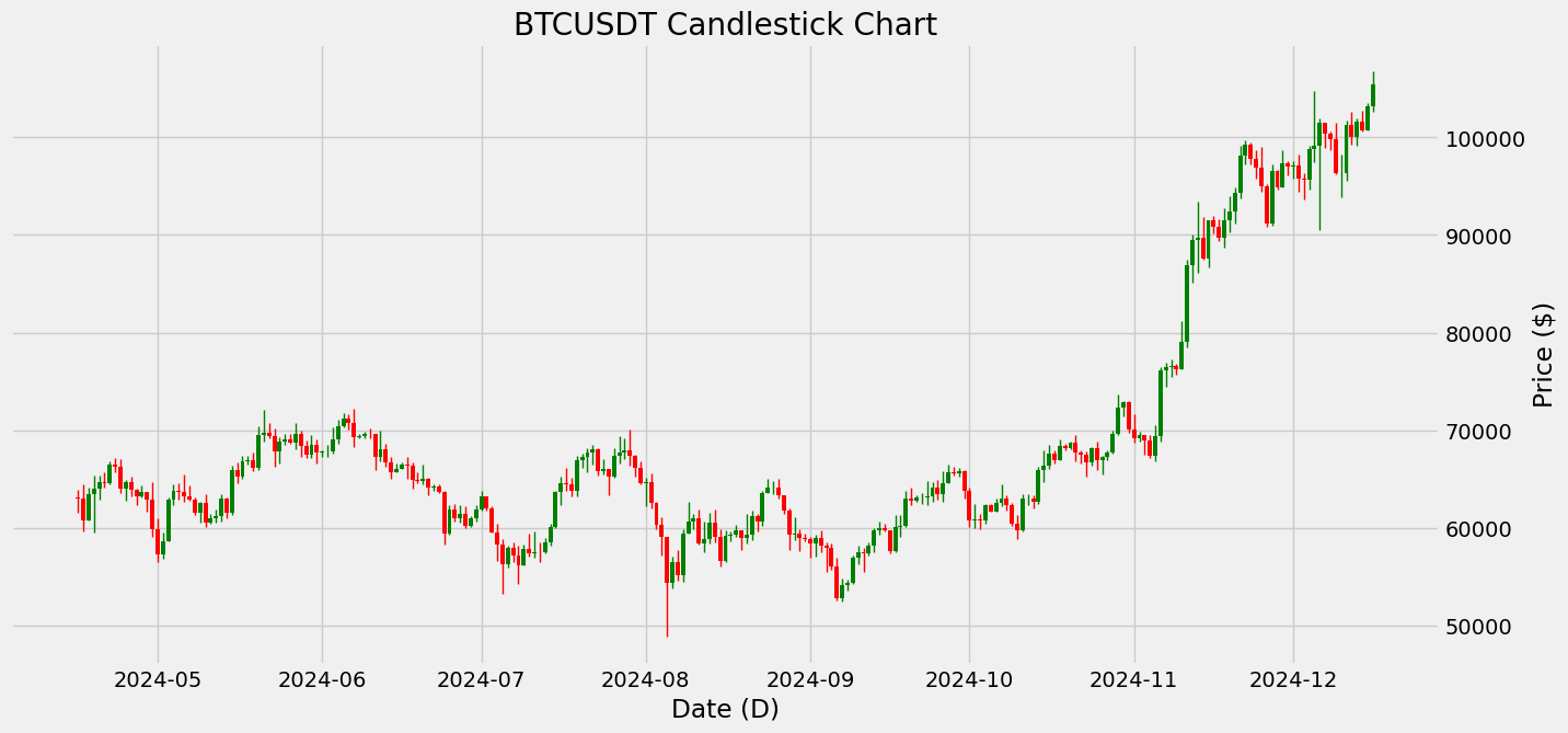
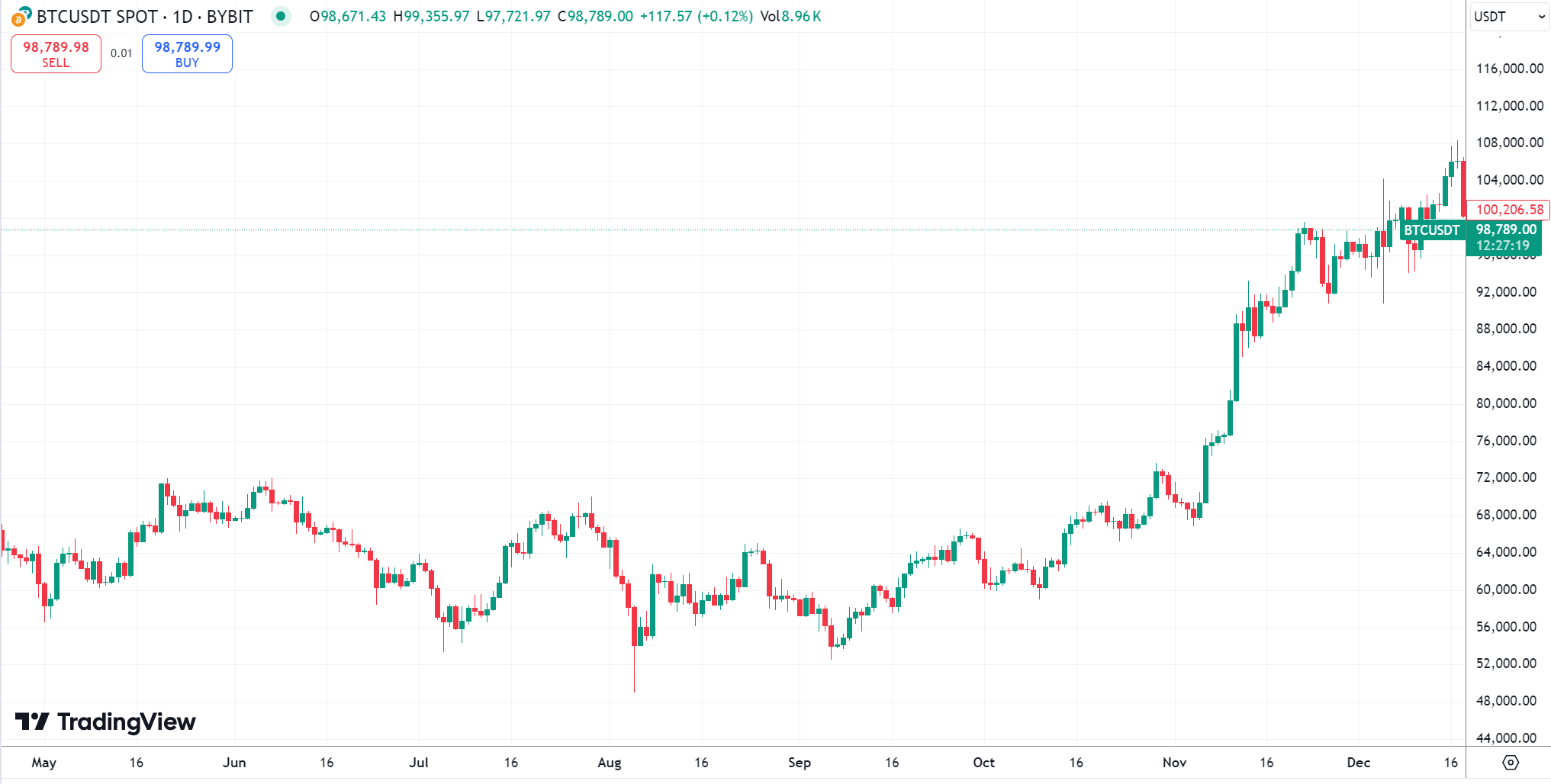
Indeed, these data are consistent with the TradingView chart.
3. Develop methods for identifying support and resistance levels
Support and resistance levels are usually determined based on previous price movements. Traders and analysts pay attention to points where the price has repeatedly stalled or reversed. Such points are considered important both psychologically and technically, as they indicate areas of interest for buyers and sellers.
Identifying local maxima and minima
Let’s attempt to design an algorithm for identifying support and resistance levels. For this, I suggest using an approach based on finding local minima and maxima. To identify local maxima and minima on a chart, a method comparing neighboring points can be applied. A local maximum is a point that is higher than its neighbors on the left and right, while a local minimum is, conversely, lower than its neighboring points.
We will use NumPy to work with arrays.
1
import numpy as np
We will create an array of prices based on the close values, removing unnecessary noise from the candles.
1
2
all_close = slice_candles['Close'].values
all_close = all_close[~np.isnan(all_close)]
Let’s try splitting our array into subarrays and finding the minimum and maximum within each. These will serve as our local minima and maxima.
1
2
3
4
5
6
7
8
9
10
11
12
13
14
15
16
17
18
19
20
21
22
23
24
25
26
27
28
29
30
31
32
33
34
dtype_dict = {
    'New_Min_Index': int,
    'New_Max_Index': int
}

def find_extr(arr, divider):
    # Split the array into subarrays
    split_arrays = np.array_split(arr, len(arr) // divider)

    data = {
        'Minimum': [],
        'Min_Index': [],
        'Maximum': [],
        'Max_Index': []
    }

    # Find the minimum and maximum in each subarray
    for i, subarray in enumerate(split_arrays):
        minimum = np.min(subarray)
        maximum = np.max(subarray)
        min_index = np.argmin(subarray) + i * divider
        max_index = np.argmax(subarray) + i * divider

        data['Minimum'].append(minimum)
        data['Min_Index'].append(min_index)
        data['Maximum'].append(maximum)
        data['Max_Index'].append(max_index)

    df = pd.DataFrame(data)
    return df

ext_price = find_extr(all_close, 30)

print(ext_price)
1
2
3
4
5
6
7
8
9
   Minimum  Min_Index   Maximum  Max_Index
0  57330.0         15   66468.5          6
1  65743.2         58   71215.0         49
2  56235.0         81   66350.0         60
3  54375.3        108   68097.3         94
4  52872.0        139   64182.8        127
5  59771.1        172   67590.4        178
6  66676.5        185   91492.8        208
7  89724.4        210  105441.6        239
We will attempt to reduce the number of points using some simple logic. By shifting the DataFrame, we will check the next row’s values. For example, the minimum of the first subarray should be smaller than the second, and the maximum should be smaller than the first subarray.
1
2
3
4
5
6
7
8
9
10
11
12
13
14
15
16
17
18
19
20
21
22
23
24
25
26
27
28
29
30
31
32
33
34
35
36
37
38
39
40
# Shift the data one row down
shifted_df = ext_price.shift()

# Condition: Minimum of the first row < Maximum of the second row
condition1 = shifted_df['Maximum'] > ext_price['Minimum']
condition2 = shifted_df['Minimum'] < ext_price['Maximum']

# Select the minimum values between the current and the next row
new_minimum = ext_price['Minimum'].combine(shifted_df['Minimum'], min).where(condition1)
new_maximum = ext_price['Maximum'].combine(shifted_df['Maximum'], max)

# Transfer indices for new values
new_min_index = ext_price['Min_Index'].where(new_minimum == ext_price['Minimum'], other=shifted_df['Min_Index'])
new_max_index = ext_price['Max_Index'].where(new_maximum == ext_price['Maximum'], other=shifted_df['Max_Index'])

# Create a new DataFrame
result = pd.DataFrame({
    'New_Minimum': new_minimum,
    'New_Min_Index': new_min_index,
    'New_Maximum': new_maximum,
    'New_Max_Index': new_max_index
})

splice_indexs = np.empty(shape=0, dtype=int)
for _, row in result.iterrows():
    if row['New_Min_Index'] > row['New_Max_Index']:
        new_values = np.array([row['New_Min_Index'], row['New_Max_Index']], dtype=int)
        splice_indexs = np.append(splice_indexs, new_values)

# Sort the array and remove duplicate elements
splice_indexs = np.unique(splice_indexs)

# Remove zero elements
splice_indexs = splice_indexs[splice_indexs != 0]

print(splice_indexs)

arrs = np.split(all_close, splice_indexs)
print(arrs)
1
2
3
4
5
6
7
8
9
10
11
12
13
14
15
16
17
18
19
20
21
22
23
24
25
26
27
28
29
30
31
32
33
34
35
[ 49  81  94 108 139]
[array([62999. , 60825.9, 63471.5, 64026.1, 64690.6, 64623.2, 66468.5,
       66329. , 64081.2, 64751. , 63949.9, 63251.9, 63650. , 62942. ,
       59933.5, 57330. , 58688.8, 62871.8, 63850.1, 63708. , 63300.6,
       62967.9, 61537.1, 62584.6, 60506.6, 60990.4, 61249.8, 63068. ,
       61584.6, 65902.4, 65258.2, 66858.5, 66944. , 66122.4, 69480.5,
       69751.8, 69472.2, 67850.3, 68840.2, 69104.8, 68730. , 69685.1,
       68367.9, 67504.3, 68477.8, 67740. , 67832. , 67840. , 69135.5]), array([70418.1, 71215. , 70770. , 69359.4, 69395. , 69689.1, 69616.6,
       67258.3, 68076.7, 66676.2, 65743.2, 66014. , 66479. , 66350. ,
       64915.8, 64855.4, 65091. , 64183.3, 64250.6, 63709.1, 59471.4,
       61879.7, 60960. , 61461.8, 60217.1, 61007. , 61942.1, 63251.3,
       61983.2, 59572. , 58337.2, 56318.5]), array([57935.5, 57244.7, 56235. , 57916.6, 57398. , 57536.7, 57510.8,
       58565. , 60063.5, 63684.7, 64634.5, 64479.9, 63803. ]), array([66903.4, 67313.3, 67699. , 68097.3, 65812.3, 66033.3, 65274. ,
       67404.8, 67790.4, 68014.5, 67347. , 66172.1, 64570.9, 64728. ]), array([62602. , 60372.4, 59124.3, 54375.3, 56515.3, 55130.1, 59457.5,
       60718.5, 60965.3, 58478.9, 58823.6, 60531.9, 59130.4, 56635.6,
       59229.2, 59370.3, 59792. , 59043.3, 59286.8, 61208.1, 60663.1,
       63580.5, 64101.2, 64182.8, 63388. , 61842.8, 59286.5, 59489.3,
       59033.8, 58922.6, 58401.1]), array([ 58953.3,  58209.8,  58005.7,  56060.8,  52872. ,  54134.1,
        54357.7,  56989.5,  57544.5,  57446. ,  58176. ,  59800. ,
        59988.4,  59770.1,  57667.1,  60090. ,  60204.6,  62988.2,
        62777.5,  63110.9,  63185.2,  63291.9,  64196.9,  63493.3,
        64620.3,  65760.1,  65616.9,  65790.7,  63781.7,  60788.4,
        60890. ,  60757.3,  62382.6,  61706. ,  62581.5,  62995.2,
        62361.7,  60391.9,  59771.1,  62978. ,  63005.7,  62738.1,
        65897.5,  66443.6,  67590.4,  66908. ,  68404.1,  68225.5,
        68760. ,  67748.8,  67512.1,  66676.5,  68162.1,  66909.9,
        67239.8,  67738. ,  69630.8,  72335. ,  72913.2,  70071.1,
        69250. ,  69541.2,  68952.5,  67356.8,  69420.5,  76110.2,
        76454.3,  76585.4,  76305. ,  79008. ,  86886.5,  89540.9,
        89724.8,  87621.2,  91492.8,  90821.5,  89724.4,  91540.1,
        92466.6,  94279.7,  98174.4,  99230.9,  97791.6,  96897.3,
        95046.8,  91124.2,  96558.2,  94888.1,  97368.8,  97035.6,
        97157.1,  95720.4,  95663.1,  98795.6,  99135. , 101450.7,
       100388.9,  99846.8,  96300. ,  96378.7, 101259.7,  99995.6,
       101650. , 100749.3, 103149.8, 105441.6])]
Visualization:
1
2
3
4
5
6
7
8
9
10
11
12
13
14
15
16
17
18
19
20
21
22
23
24
25
26
27
28
29
30
31
32
33
34
35
36
37
38
39
40
41
42
43
44
45
46
47
48
49
50
51
52
def draw_chart(arrs, chart_title="Subarray"):
    """
    Function to display a chart of subarrays with annotations for minimum and maximum values.

    Parameters:
    arrs (list): List of subarrays to display.
    chart_title (str): Title of the chart.
    """
    # Set up chart parameters
    fig, ax = plt.subplots(figsize=(12, 6))
    plt.style.use('fivethirtyeight')

    # Move the y-axis ticks and labels to the right
    ax.yaxis.tick_right()
    ax.yaxis.set_label_position('right')
    ax.set_xlabel('Array Elements')
    ax.set_ylabel('Price')
    ax.set_title(chart_title)

    offset = 0  # Offset for each subarray
    for i, subarray in enumerate(arrs):
        if len(subarray) == 0:  # Check for empty arrays
            continue  # Skip empty arrays

        x = np.arange(len(subarray)) + offset
        ax.plot(x, subarray, label=f'Arr {i+1}', linewidth=2)

        # Add points for minimum and maximum values
        min_index = np.argmin(subarray)
        max_index = np.argmax(subarray)
        min_value = subarray[min_index]
        max_value = subarray[max_index]

        # Annotate the minimum and maximum points on the chart
        ax.scatter(x[min_index], min_value, color='red', zorder=5)
        ax.scatter(x[max_index], max_value, color='green', zorder=5)

        offset += len(subarray)  # Update offset for the next subarray

    # Add legend and grid
    ax.legend()
    ax.grid(True)

    # Add descriptions for red and green points
    ax.text(0.98, 0.98, "Local minimum", transform=ax.transAxes,
            fontsize=12, color='red', va='top', ha='right')
    ax.text(0.98, 0.94, "Local maximum", transform=ax.transAxes,
            fontsize=12, color='green', va='top', ha='right')

    # Show the chart
    plt.show()
1
draw_chart(arrs)
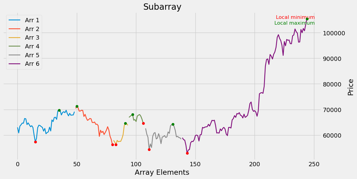
We’ll now attempt to divide the chart into waves by connecting the minimum and maximum points of two subarrays. To achieve this, we’ll enhance our function to handle shifting the array while dividing it into subarrays.
1
2
3
4
5
6
7
8
9
10
11
12
13
14
15
16
17
18
19
20
21
22
23
24
25
26
27
28
29
30
31
32
33
34
35
36
37
38
39
40
41
42
def find_extr(arr, divider, shift):
    """
    Divides an array into subarrays with a given divider and shift, then finds extremum points.

    Parameters:
    arr (np.array): Input array.
    divider (int): Size of each subarray.
    shift (int): Shift for dividing subarrays.

    Returns:
    pd.DataFrame: DataFrame with minimums, maximums, and their indices.
    """
    data = {
        'Minimum': [],
        'Min_Index': [],
        'Maximum': [],
        'Max_Index': []
    }

    # Divide the array with a shift
    for start in range(0, len(arr) - divider + 1, shift):
        subarray = arr[start:start + divider]
        minimum = np.min(subarray)
        maximum = np.max(subarray)
        min_index = np.argmin(subarray) + start
        max_index = np.argmax(subarray) + start

        data['Minimum'].append(minimum)
        data['Min_Index'].append(min_index)
        data['Maximum'].append(maximum)
        data['Max_Index'].append(max_index)

    # Convert results into a DataFrame
    local_df = pd.DataFrame(data)
    return local_df

# Example usage
divider = 30
shift = 20

result = find_extr(all_close, divider, shift)
print(result)
1
2
3
4
5
6
7
8
9
10
11
12
    Minimum  Min_Index  Maximum  Max_Index
0   57330.0         15  66468.5          6
1   60506.6         24  70418.1         49
2   59471.4         69  71215.0         50
3   56235.0         83  66479.0         61
4   56235.0         83  68097.3         97
5   54375.3        111  68014.5        103
6   52872.0        143  64182.8        131
7   52872.0        143  65790.7        166
8   59771.1        177  68760.0        187
9   62738.1        180  86886.5        209
10  67356.8        202  99230.9        220
Let’s try a new method.
1
2
3
4
5
divider = 30
shift = 20

result = find_extr(all_close, divider, shift)
print(result)
1
2
3
4
5
6
7
8
9
10
11
12
    Minimum  Min_Index  Maximum  Max_Index
0   57330.0         15  66468.5          6
1   60506.6         24  70418.1         49
2   59471.4         69  71215.0         50
3   56235.0         83  66479.0         61
4   56235.0         83  68097.3         97
5   54375.3        111  68014.5        103
6   52872.0        143  64182.8        131
7   52872.0        143  65790.7        166
8   59771.1        177  68760.0        187
9   62738.1        180  86886.5        209
10  67356.8        202  99230.9        220
We will also put the verified code in the function
1
2
3
4
5
6
7
8
9
10
11
12
13
14
15
16
17
18
19
20
21
22
23
24
25
26
27
28
29
30
31
32
33
34
35
36
37
38
39
40
41
42
43
44
45
46
47
48
49
50
51
52
53
54
55
56
57
def process_extreme_values(ext_price):
    """
    Processes extremum values in a DataFrame using a shift.

    Parameters:
    ext_price (pd.DataFrame): DataFrame with extremum data for processing.

    Returns:
    pd.DataFrame: DataFrame with new minimums, maximums, and their indices.
    np.array: Array of split indices for dividing the array into subarrays.
    """
    # Shift data one row down
    shifted_df = ext_price.shift()

    # Condition: Minimum of the first row < Maximum of the second row
    condition1 = shifted_df['Maximum'] > ext_price['Minimum']
    condition2 = shifted_df['Minimum'] < ext_price['Maximum']

    # Select minimum values between the current and the next row
    new_minimum = ext_price['Minimum'].combine(shifted_df['Minimum'], min).where(condition1)
    new_maximum = ext_price['Maximum'].combine(shifted_df['Maximum'], max)

    # Transfer indices for new values
    new_min_index = ext_price['Min_Index'].where(new_minimum == ext_price['Minimum'], other=shifted_df['Min_Index'])
    new_max_index = ext_price['Max_Index'].where(new_maximum == ext_price['Maximum'], other=shifted_df['Max_Index'])

    # Create a new DataFrame
    result = pd.DataFrame({
        'New_Minimum': new_minimum,
        'New_Min_Index': new_min_index,
        'New_Maximum': new_maximum,
        'New_Max_Index': new_max_index
    })

    # Process indices for splits
    splice_indexs = np.empty(shape=0, dtype=int)
    for _, row in result.iterrows():
        if row['New_Min_Index'] > row['New_Max_Index']:
            new_values = np.array([row['New_Min_Index'], row['New_Max_Index']], dtype=int)
            splice_indexs = np.append(splice_indexs, new_values)

    # Sort the array and remove duplicate elements
    splice_indexs = np.unique(splice_indexs)

    return result, splice_indexs

# Example usage
result_df, splice_indices = process_extreme_values(result)

# Output results
print("Result DataFrame:")
print(result_df)

# Example of working with `arrs` using `splice_indices` to split data
arrs = np.split(all_close, splice_indices)
print("Split arrays:", arrs)
1
2
3
4
5
6
7
8
9
10
11
12
13
14
15
16
17
18
19
20
21
22
23
24
25
26
27
28
29
30
31
32
33
34
35
36
37
38
39
40
41
42
43
44
45
46
Result DataFrame:
    New_Minimum  New_Min_Index  New_Maximum  New_Max_Index
0           NaN            NaN      66468.5              6
1       57330.0           15.0      70418.1             49
2       59471.4           69.0      71215.0             50
3       56235.0           83.0      71215.0             50
4       56235.0           83.0      68097.3             97
5       54375.3          111.0      68097.3             97
6       52872.0          143.0      68014.5            103
7       52872.0          143.0      65790.7            166
8       52872.0          143.0      68760.0            187
9       59771.1          177.0      86886.5            209
10      62738.1          180.0      99230.9            220
Split arrays: [array([62999. , 60825.9, 63471.5, 64026.1, 64690.6, 64623.2, 66468.5,
       66329. , 64081.2, 64751. , 63949.9, 63251.9, 63650. , 62942. ,
       59933.5, 57330. , 58688.8, 62871.8, 63850.1, 63708. , 63300.6,
       62967.9, 61537.1, 62584.6, 60506.6, 60990.4, 61249.8, 63068. ,
       61584.6, 65902.4, 65258.2, 66858.5, 66944. , 66122.4, 69480.5,
       69751.8, 69472.2, 67850.3, 68840.2, 69104.8, 68730. , 69685.1,
       68367.9, 67504.3, 68477.8, 67740. , 67832. , 67840. , 69135.5,
       70418.1]), array([71215. , 70770. , 69359.4, 69395. , 69689.1, 69616.6, 67258.3,
       68076.7, 66676.2, 65743.2, 66014. , 66479. , 66350. , 64915.8,
       64855.4, 65091. , 64183.3, 64250.6, 63709.1]), array([59471.4, 61879.7, 60960. , 61461.8, 60217.1, 61007. , 61942.1,
       63251.3, 61983.2, 59572. , 58337.2, 56318.5, 57935.5, 57244.7]), array([56235. , 57916.6, 57398. , 57536.7, 57510.8, 58565. , 60063.5,
       63684.7, 64634.5, 64479.9, 63803. , 66903.4, 67313.3, 67699. ]), array([68097.3, 65812.3, 66033.3, 65274. , 67404.8, 67790.4]), array([68014.5, 67347. , 66172.1, 64570.9, 64728. , 62602. , 60372.4,
       59124.3]), array([54375.3, 56515.3, 55130.1, 59457.5, 60718.5, 60965.3, 58478.9,
       58823.6, 60531.9, 59130.4, 56635.6, 59229.2, 59370.3, 59792. ,
       59043.3, 59286.8, 61208.1, 60663.1, 63580.5, 64101.2, 64182.8,
       63388. , 61842.8, 59286.5, 59489.3, 59033.8, 58922.6, 58401.1,
       58953.3, 58209.8, 58005.7, 56060.8]), array([ 52872. ,  54134.1,  54357.7,  56989.5,  57544.5,  57446. ,
        58176. ,  59800. ,  59988.4,  59770.1,  57667.1,  60090. ,
        60204.6,  62988.2,  62777.5,  63110.9,  63185.2,  63291.9,
        64196.9,  63493.3,  64620.3,  65760.1,  65616.9,  65790.7,
        63781.7,  60788.4,  60890. ,  60757.3,  62382.6,  61706. ,
        62581.5,  62995.2,  62361.7,  60391.9,  59771.1,  62978. ,
        63005.7,  62738.1,  65897.5,  66443.6,  67590.4,  66908. ,
        68404.1,  68225.5,  68760. ,  67748.8,  67512.1,  66676.5,
        68162.1,  66909.9,  67239.8,  67738. ,  69630.8,  72335. ,
        72913.2,  70071.1,  69250. ,  69541.2,  68952.5,  67356.8,
        69420.5,  76110.2,  76454.3,  76585.4,  76305. ,  79008. ,
        86886.5,  89540.9,  89724.8,  87621.2,  91492.8,  90821.5,
        89724.4,  91540.1,  92466.6,  94279.7,  98174.4,  99230.9,
        97791.6,  96897.3,  95046.8,  91124.2,  96558.2,  94888.1,
        97368.8,  97035.6,  97157.1,  95720.4,  95663.1,  98795.6,
        99135. , 101450.7, 100388.9,  99846.8,  96300. ,  96378.7,
       101259.7,  99995.6, 101650. , 100749.3, 103149.8, 105441.6])]
Getting the sub-arrays.
1
2
3
4
5
6
7
8
9
10
# Function call
result_df, splice_indices = process_extreme_values(result)

# Output of results
print("Result DataFrame:")
print(result_df)

# Splitting the array by indexes
arrs = np.split(all_close, splice_indices)
print("Split arrays:", arrs)
1
2
3
4
5
6
7
8
9
10
11
12
13
14
15
16
17
18
19
20
21
22
23
24
25
26
27
28
29
30
31
32
33
34
35
36
37
38
39
40
41
42
43
44
45
46
Result DataFrame:
    New_Minimum  New_Min_Index  New_Maximum  New_Max_Index
0           NaN            NaN      66468.5              6
1       57330.0           15.0      70418.1             49
2       59471.4           69.0      71215.0             50
3       56235.0           83.0      71215.0             50
4       56235.0           83.0      68097.3             97
5       54375.3          111.0      68097.3             97
6       52872.0          143.0      68014.5            103
7       52872.0          143.0      65790.7            166
8       52872.0          143.0      68760.0            187
9       59771.1          177.0      86886.5            209
10      62738.1          180.0      99230.9            220
Split arrays: [array([62999. , 60825.9, 63471.5, 64026.1, 64690.6, 64623.2, 66468.5,
       66329. , 64081.2, 64751. , 63949.9, 63251.9, 63650. , 62942. ,
       59933.5, 57330. , 58688.8, 62871.8, 63850.1, 63708. , 63300.6,
       62967.9, 61537.1, 62584.6, 60506.6, 60990.4, 61249.8, 63068. ,
       61584.6, 65902.4, 65258.2, 66858.5, 66944. , 66122.4, 69480.5,
       69751.8, 69472.2, 67850.3, 68840.2, 69104.8, 68730. , 69685.1,
       68367.9, 67504.3, 68477.8, 67740. , 67832. , 67840. , 69135.5,
       70418.1]), array([71215. , 70770. , 69359.4, 69395. , 69689.1, 69616.6, 67258.3,
       68076.7, 66676.2, 65743.2, 66014. , 66479. , 66350. , 64915.8,
       64855.4, 65091. , 64183.3, 64250.6, 63709.1]), array([59471.4, 61879.7, 60960. , 61461.8, 60217.1, 61007. , 61942.1,
       63251.3, 61983.2, 59572. , 58337.2, 56318.5, 57935.5, 57244.7]), array([56235. , 57916.6, 57398. , 57536.7, 57510.8, 58565. , 60063.5,
       63684.7, 64634.5, 64479.9, 63803. , 66903.4, 67313.3, 67699. ]), array([68097.3, 65812.3, 66033.3, 65274. , 67404.8, 67790.4]), array([68014.5, 67347. , 66172.1, 64570.9, 64728. , 62602. , 60372.4,
       59124.3]), array([54375.3, 56515.3, 55130.1, 59457.5, 60718.5, 60965.3, 58478.9,
       58823.6, 60531.9, 59130.4, 56635.6, 59229.2, 59370.3, 59792. ,
       59043.3, 59286.8, 61208.1, 60663.1, 63580.5, 64101.2, 64182.8,
       63388. , 61842.8, 59286.5, 59489.3, 59033.8, 58922.6, 58401.1,
       58953.3, 58209.8, 58005.7, 56060.8]), array([ 52872. ,  54134.1,  54357.7,  56989.5,  57544.5,  57446. ,
        58176. ,  59800. ,  59988.4,  59770.1,  57667.1,  60090. ,
        60204.6,  62988.2,  62777.5,  63110.9,  63185.2,  63291.9,
        64196.9,  63493.3,  64620.3,  65760.1,  65616.9,  65790.7,
        63781.7,  60788.4,  60890. ,  60757.3,  62382.6,  61706. ,
        62581.5,  62995.2,  62361.7,  60391.9,  59771.1,  62978. ,
        63005.7,  62738.1,  65897.5,  66443.6,  67590.4,  66908. ,
        68404.1,  68225.5,  68760. ,  67748.8,  67512.1,  66676.5,
        68162.1,  66909.9,  67239.8,  67738. ,  69630.8,  72335. ,
        72913.2,  70071.1,  69250. ,  69541.2,  68952.5,  67356.8,
        69420.5,  76110.2,  76454.3,  76585.4,  76305. ,  79008. ,
        86886.5,  89540.9,  89724.8,  87621.2,  91492.8,  90821.5,
        89724.4,  91540.1,  92466.6,  94279.7,  98174.4,  99230.9,
        97791.6,  96897.3,  95046.8,  91124.2,  96558.2,  94888.1,
        97368.8,  97035.6,  97157.1,  95720.4,  95663.1,  98795.6,
        99135. , 101450.7, 100388.9,  99846.8,  96300. ,  96378.7,
       101259.7,  99995.6, 101650. , 100749.3, 103149.8, 105441.6])]
1
draw_chart(arrs)
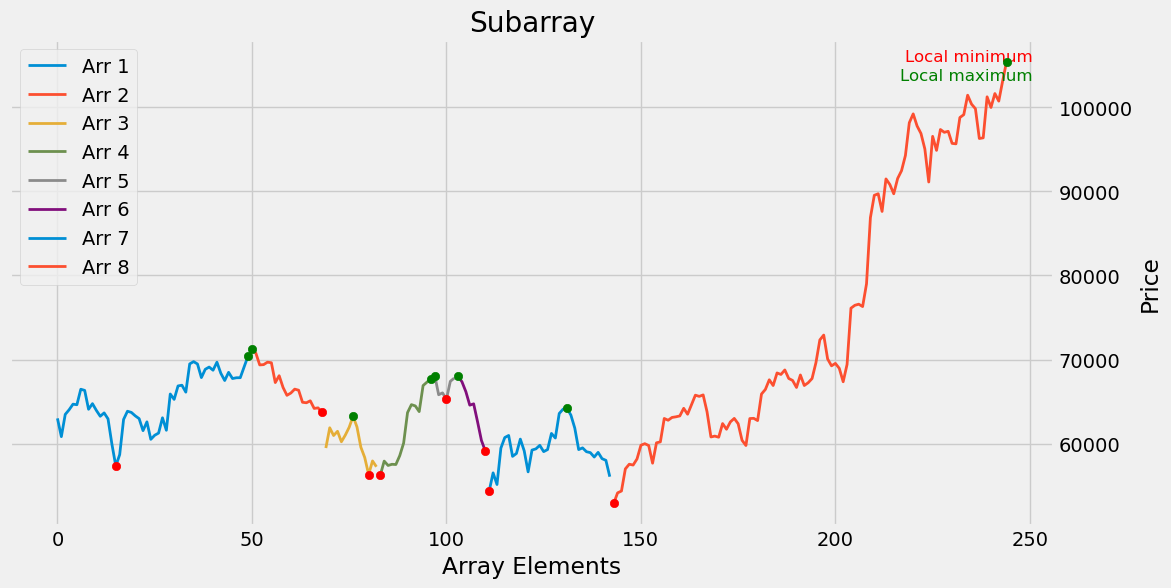
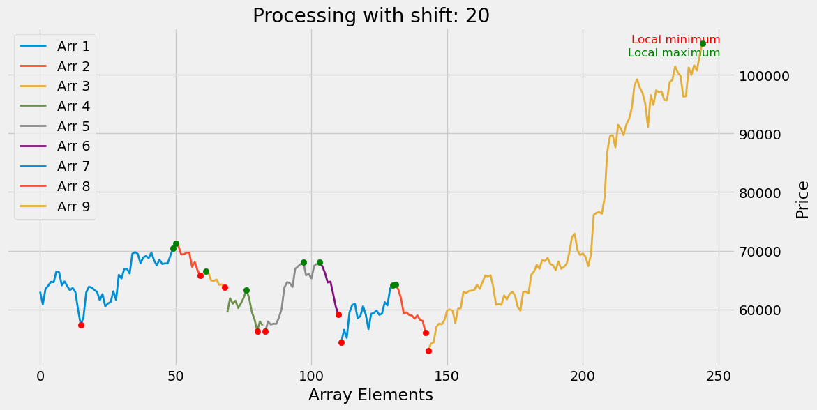
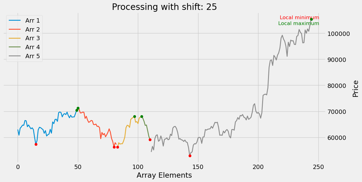
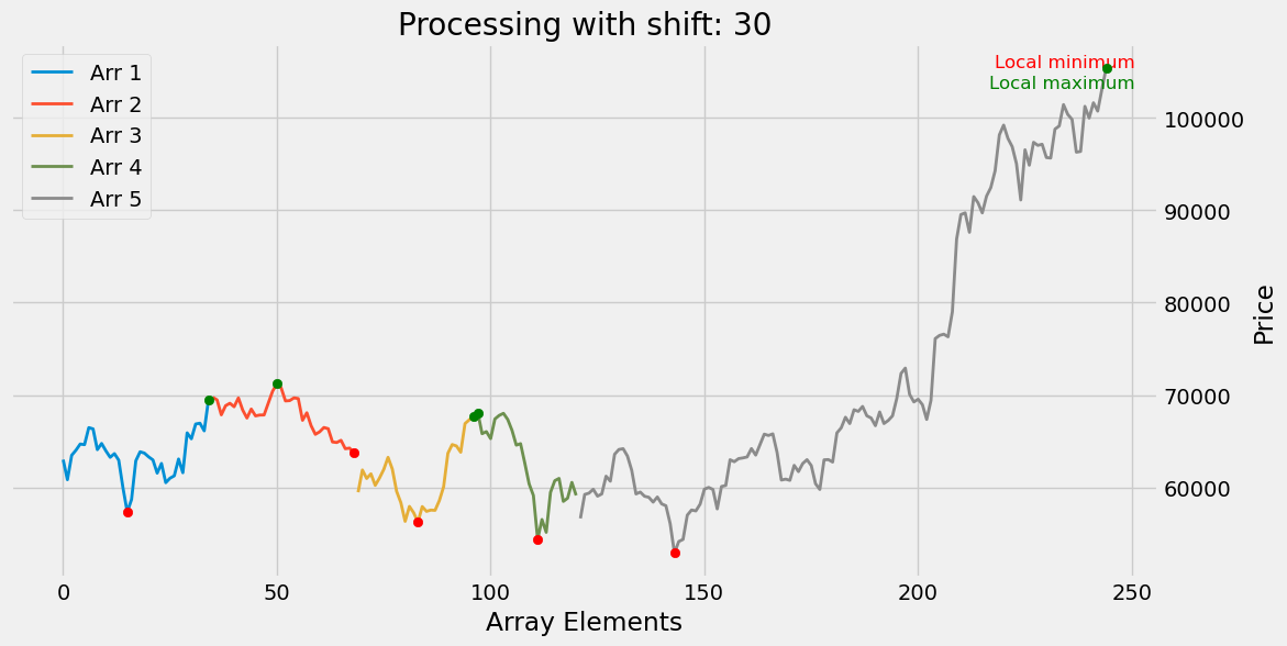
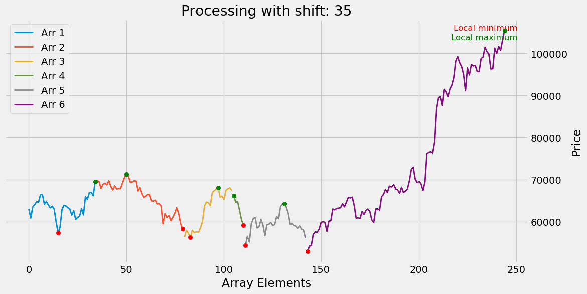
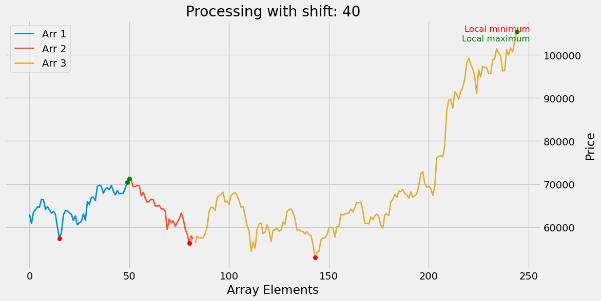
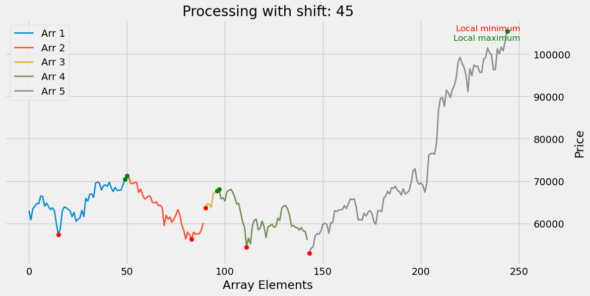
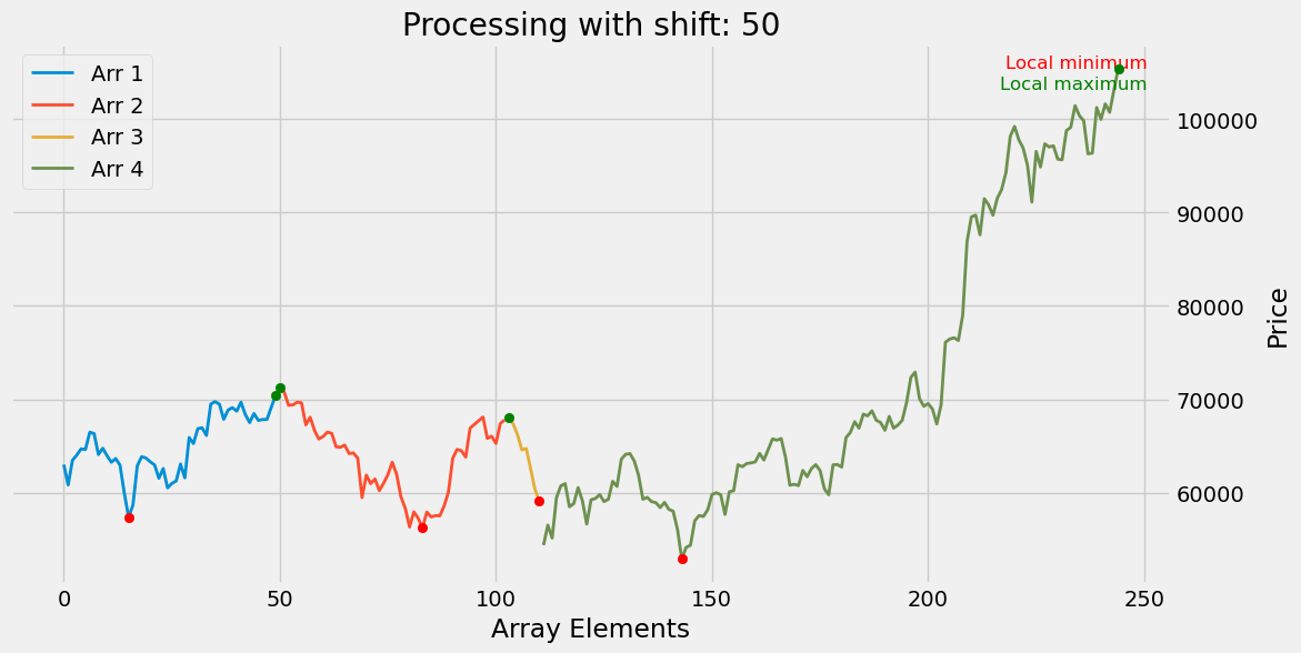
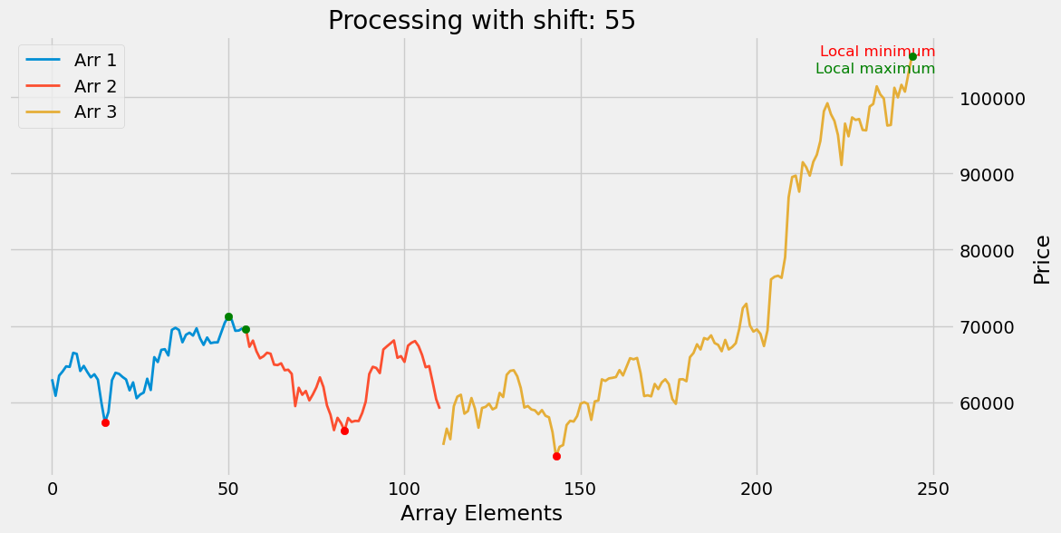
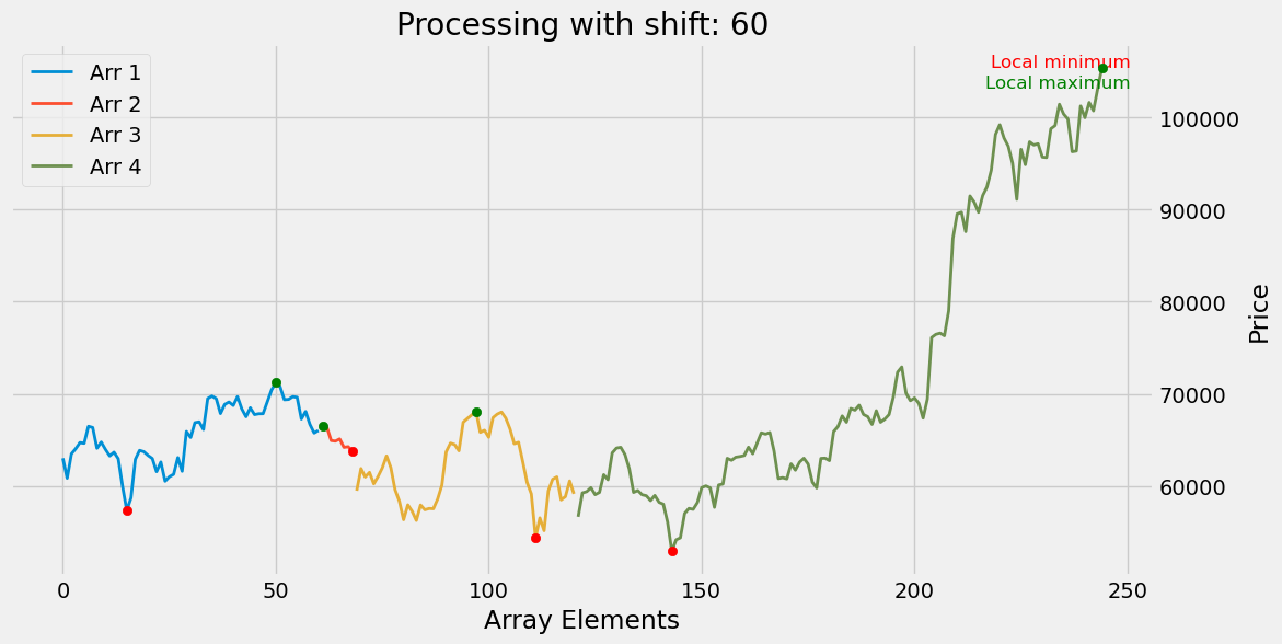
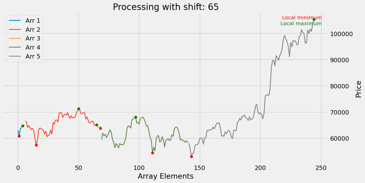
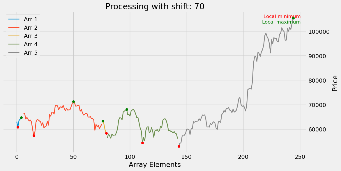
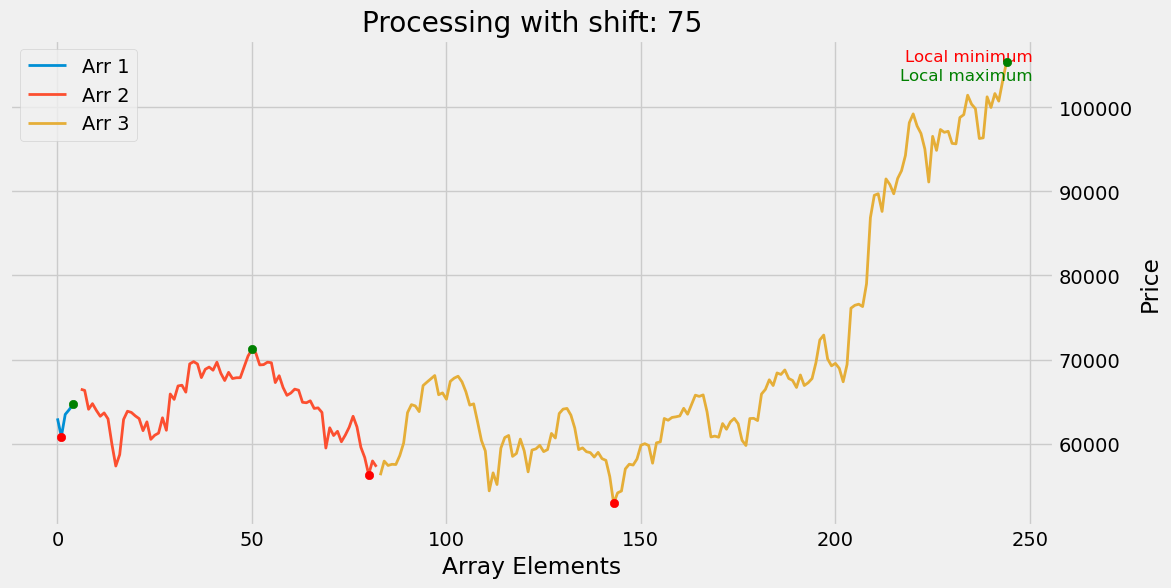
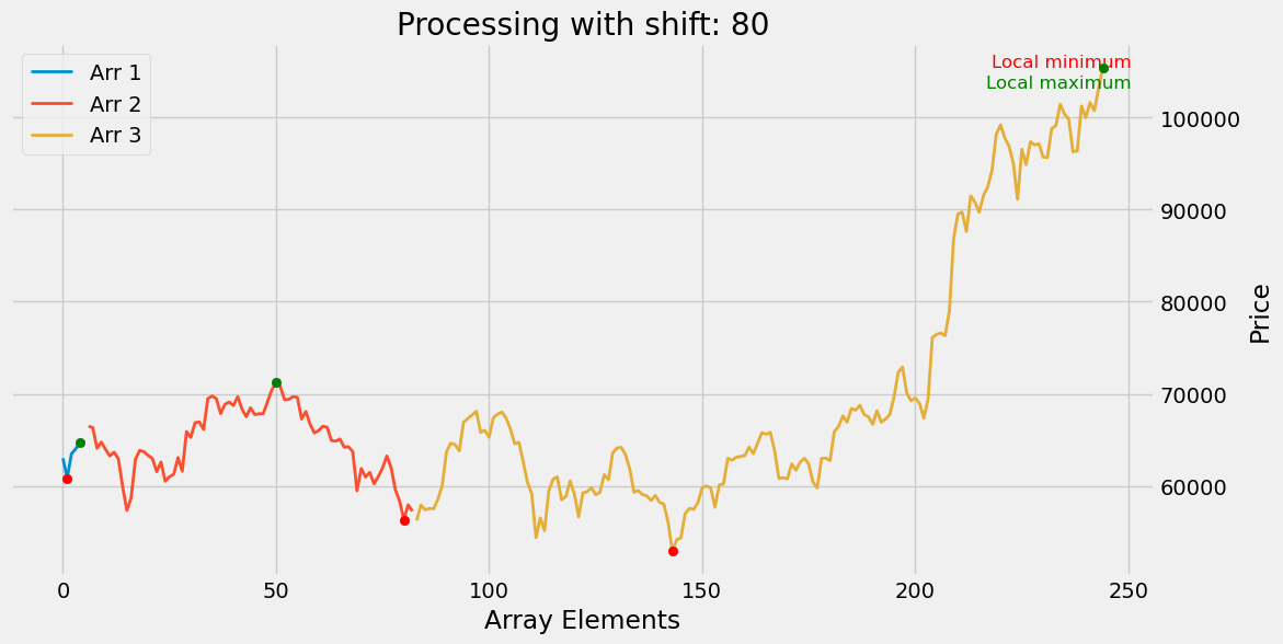
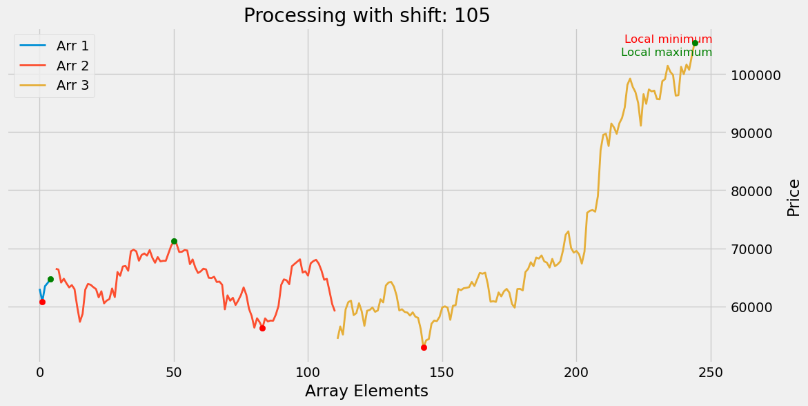
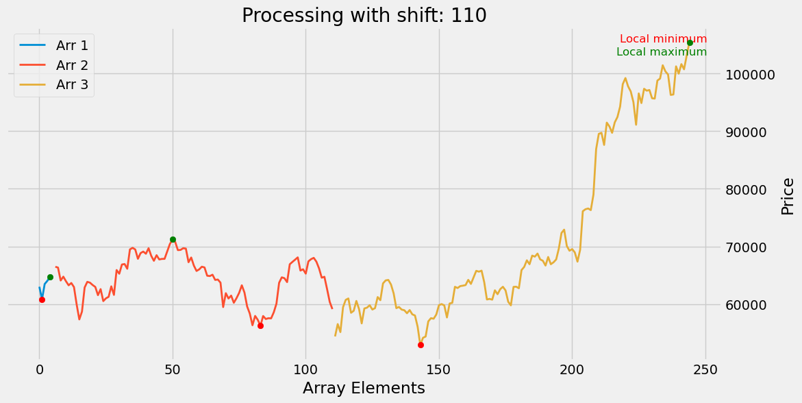
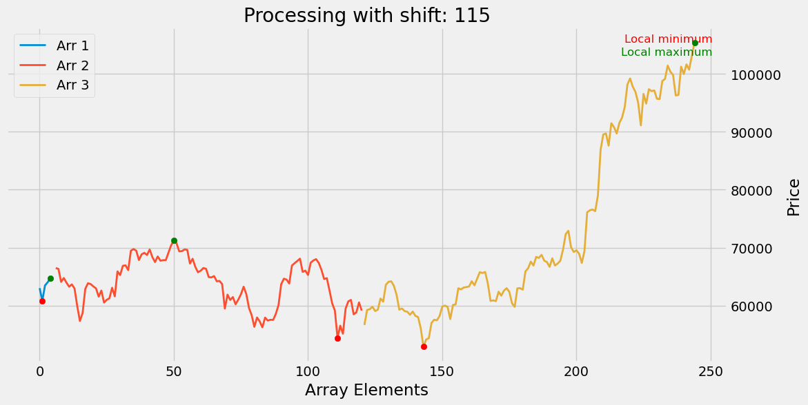
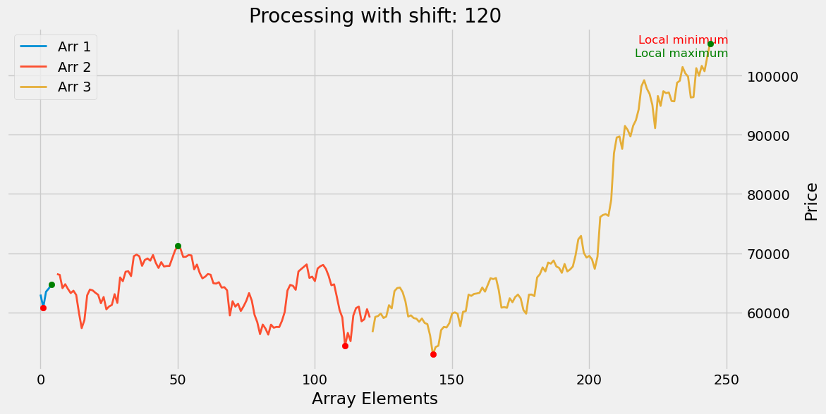
Consider the scenario of an array displacement and investigate the possibility of matching the position of the extreme points.
1
2
3
4
5
6
7
8
9
10
11
12
13
14
15
16
17
18
19
20
21
22
23
24
25
26
27
28
29
30
31
32
33
34
35
36
37
38
39
40
41
divider = len(all_close) // 20  # Block size
shift_increment = 5  # Shift increment
max_shift = len(all_close) // 2  # Maximum shift
# print(divider)

# Empty list to store DataFrame rows
rows = []

# Loop through varying shifts
for shift in range(20, max_shift, shift_increment):
    print(f"Processing with shift: {shift}")

    # Get extrema and indices for splitting
    result_df, splice_indices = process_extreme_values(find_extr(all_close, divider, shift))

    # Split data into subarrays
    arrs = np.split(all_close, splice_indices)

    # Process each subarray
    for i, subarray in enumerate(arrs):
        if subarray.size == 0:
            continue  # Skip empty subarray

        # Find minimum and maximum values for the subarray
        min_value = np.min(subarray)
        max_value = np.max(subarray)

        # Add a row to the list
        rows.append({
            'Shift': shift,
            'Array': i+1,
            'Min': min_value,
            'Max': max_value
        })

    # Plot graphs
    draw_chart(arrs, 'Processing with shift: ' + str(shift))

# Create a DataFrame from the list of rows
arr_count = pd.DataFrame(rows)
1
Processing with shift: 20
1
Processing with shift: 25
1
Processing with shift: 30
1
Processing with shift: 35
1
Processing with shift: 40
1
Processing with shift: 45
1
Processing with shift: 50
1
Processing with shift: 55
1
Processing with shift: 60
1
Processing with shift: 65
1
Processing with shift: 70
1
Processing with shift: 75
1
Processing with shift: 80
1
Processing with shift: 85
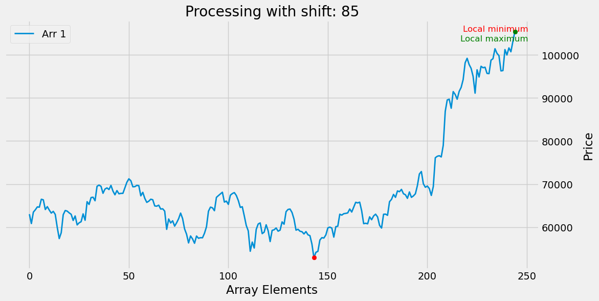
1
Processing with shift: 90
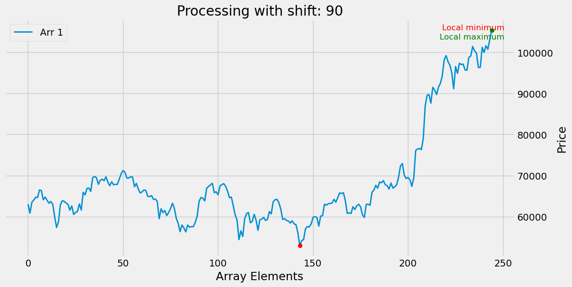
1
Processing with shift: 95
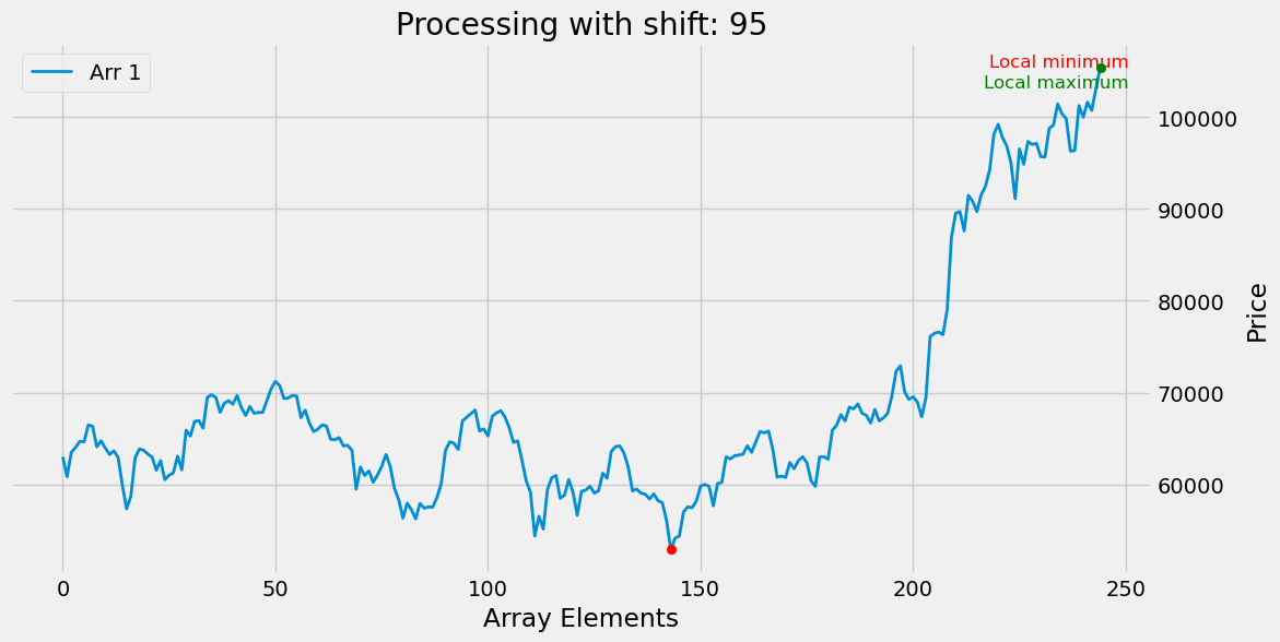
1
Processing with shift: 100
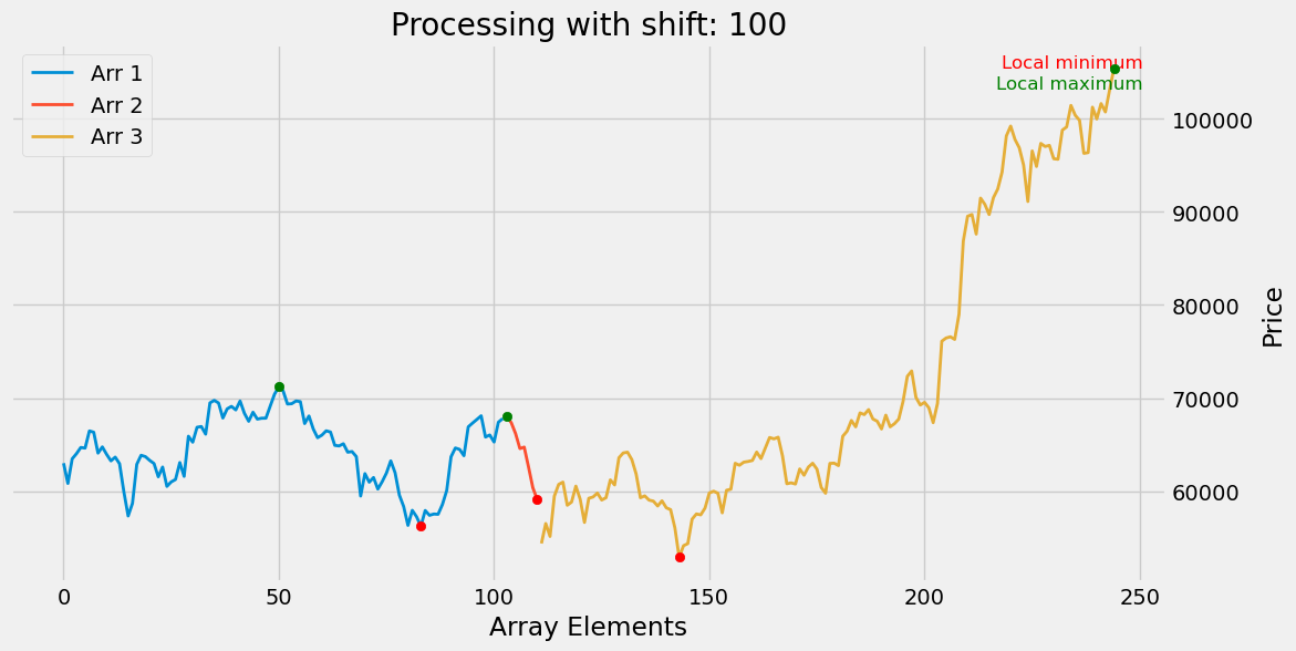
1
Processing with shift: 105
1
Processing with shift: 110
1
Processing with shift: 115
1
Processing with shift: 120
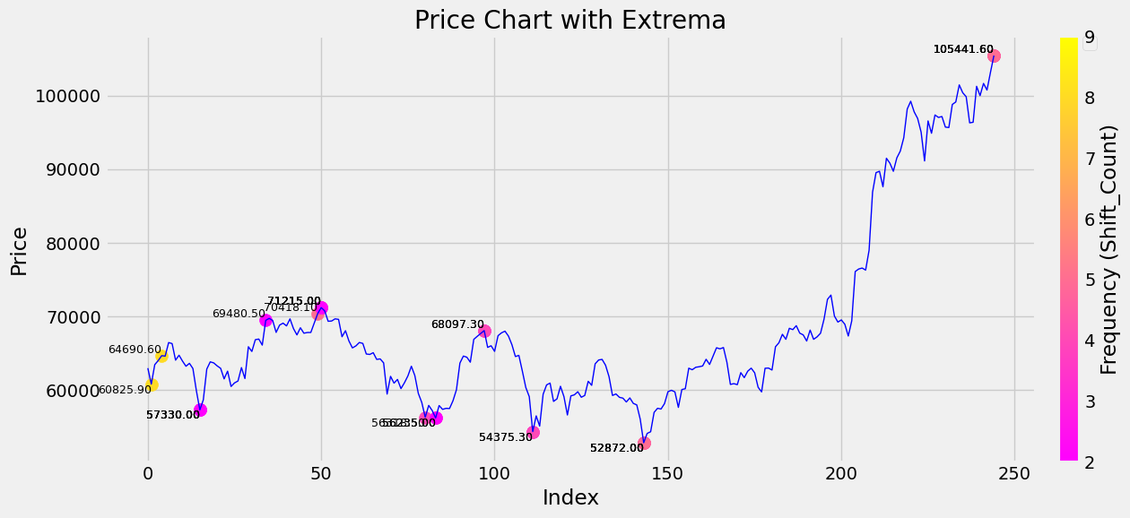
Let’s try to count how many arrays contain the same prices. This will help identify the exact min and max points. We will group the rows and count using pandas.
1
2
3
4
5
6
7
8
9
10
11
12
arr_count

# Group by Array, Min, and Max to find matches
grouped = arr_count.groupby(['Array', 'Min', 'Max'])

# Count the number of unique Shifts for each group
result = grouped['Shift'].nunique().reset_index(name='Shift_Count')

# Filter only those groups where Shift_Count > 1 (same Array, Min, and Max for different Shifts)
matches = result[result['Shift_Count'] > 1].copy()

print(matches)
1
2
3
4
5
6
7
8
9
10
11
12
13
14
15
    Array      Min       Max  Shift_Count
0       1  52872.0  105441.6            3
2       1  57330.0   69480.5            2
3       1  57330.0   70418.1            5
4       1  57330.0   71215.0            2
5       1  60825.9   64690.6            8
6       2  54375.3   71215.0            2
8       2  56235.0   71215.0            4
9       2  56318.5   71215.0            4
10      2  57330.0   71215.0            2
16      3  52872.0  105441.6            9
19      3  56235.0   68097.3            2
25      4  52872.0  105441.6            2
26      4  54375.3   68097.3            4
30      5  52872.0  105441.6            5
Add a module for plotting with a color map
1
2
from matplotlib import colormaps
from matplotlib.colors import Normalize
1
2
3
4
5
6
7
8
9
10
11
12
13
14
15
16
17
18
19
20
21
22
23
24
25
26
27
28
29
30
31
32
33
34
35
36
37
38
39
40
41
42
43
44
45
46
47
48
49
50
# Price chart
fig, ax = plt.subplots(figsize=(14, 6))  # Create ax object
ax.plot(all_close, color='blue', linewidth=1)

# Create normalization for the color scale
norm = Normalize(vmin=matches['Shift_Count'].min(), vmax=matches['Shift_Count'].max())
cmap = colormaps['spring']  # Use the new method to get cmap

# Add extrema from matches to the chart
for _, row in matches.iterrows():
    # Find indices of minimum and maximum values using np.where
    min_idx = np.where(all_close == row['Min'])[0][0]  # Index of the minimum value
    max_idx = np.where(all_close == row['Max'])[0][0]  # Index of the maximum value

    # Display the minimum value
    ax.scatter(min_idx, row['Min'], color=cmap(norm(row['Shift_Count'])), s=100)

    # Display the maximum value
    ax.scatter(max_idx, row['Max'], color=cmap(norm(row['Shift_Count'])), s=100)

    # Add labels near extrema
    ax.text(min_idx, row['Min'], f'{row["Min"]:.2f}', color='black', fontsize=9, ha='right', va='top')
    ax.text(max_idx, row['Max'], f'{row["Max"]:.2f}', color='black', fontsize=9, ha='right', va='bottom')

# Add a color scale bar
sm = plt.cm.ScalarMappable(cmap=cmap, norm=norm)
sm.set_array([])

# Specify the ax object for the color bar
cbar = plt.colorbar(sm, ax=ax, pad=0.02)  # pad increases the distance between the chart and the scale
cbar.set_label('Frequency (Shift_Count)')

# Chart settings
ax.set_title('Price Chart with Extrema')
ax.set_xlabel('Index')
ax.set_ylabel('Price')

# Legend, prevent duplicate labels
handles, labels = ax.get_legend_handles_labels()
by_label = dict(zip(labels, handles))
ax.legend(by_label.values(), by_label.keys(), loc='upper left', bbox_to_anchor=(1.05, 1), borderaxespad=0.)

# Add a grid
ax.grid(True)

# Optimize the layout of the chart elements
plt.tight_layout()

# Display the chart
plt.show()
Clustering Analysis
Here, we apply clustering techniques to identify recurring price levels and validate their significance using visual and statistical methods.
1
2
3
4
5
6
7
8
9
10
11
12
13
14
15
16
17
18
19
20
21
22
23
24
25
26
27
28
29
30
31
32
33
34
35
36
37
38
39
40
41
42
43
# Combine all Min and Max values into one array
all_values = np.concatenate([matches['Min'].values, matches['Max'].values])

# Calculate the standard deviation for all values
std_dev = np.std(all_values)

# Optionally, use the mean value to vary the threshold:
mean_value = np.mean(all_values)

# Set the threshold based on the standard deviation (e.g., 1 standard deviation)
threshold = 0.5 * std_dev  # You can use any value, such as 0.5 * std_dev for a stricter threshold

# Output the threshold for verification
print(f"Automatically calculated threshold: {threshold:.2f}")

# Sort all values
sorted_values = np.sort(all_values)

# Array to store cluster labels
clusters = []
current_cluster = []

# Clustering process
for value in sorted_values:
    if not current_cluster:
        current_cluster.append(value)
    else:
        # If the current number is close to the previous one (based on the threshold), add it to the current cluster
        if value - current_cluster[-1] <= threshold:
            current_cluster.append(value)
        else:
            # If the number is far from the previous one, save the current cluster and start a new one
            clusters.append(current_cluster)
            current_cluster = [value]

# Add the last cluster
if current_cluster:
    clusters.append(current_cluster)

# Print the results
print("Clusters of numbers (close to each other):")
for idx, cluster in enumerate(clusters, start=1):
    print(f"Cluster {idx}: {cluster}")
1
2
3
4
Automatically calculated threshold: 8389.86
Clusters of numbers (close to each other):
Cluster 1: [52872.0, 52872.0, 52872.0, 52872.0, 54375.3, 54375.3, 56235.0, 56235.0, 56318.5, 57330.0, 57330.0, 57330.0, 57330.0, 60825.9, 64690.6, 68097.3, 68097.3, 69480.5, 70418.1, 71215.0, 71215.0, 71215.0, 71215.0, 71215.0]
Cluster 2: [105441.6, 105441.6, 105441.6, 105441.6]
Calculate levels and visualize them
1
2
3
4
5
6
7
8
9
10
11
12
13
14
15
16
17
18
19
20
21
22
23
24
25
26
27
28
29
30
# Calculate the mean value for each cluster
cluster_means = [np.mean(cluster) for cluster in clusters]

# Plot the chart
fig, ax = plt.subplots(figsize=(12, 6))

# Plot the price chart (or other data)
ax.plot(all_close, label='Price (Close)', color='blue', linewidth=1)

# Add horizontal lines for each cluster
for mean in cluster_means:
    ax.axhline(mean, color='orange', linestyle='--', label=f'Cluster mean: {mean:.2f}', linewidth=width_line)

# Chart settings
ax.set_title('Price chart with found levels')
ax.set_xlabel('Index')
ax.set_ylabel('Price')

# Add a legend (to avoid duplicate labels)
handles, labels = ax.get_legend_handles_labels()
by_label = dict(zip(labels, handles))
ax.legend(by_label.values(), by_label.keys(), loc='upper left', bbox_to_anchor=(1.05, 1), borderaxespad=0.)

# Add a grid
ax.grid(True)

# Show the chart
plt.tight_layout()
plt.show()
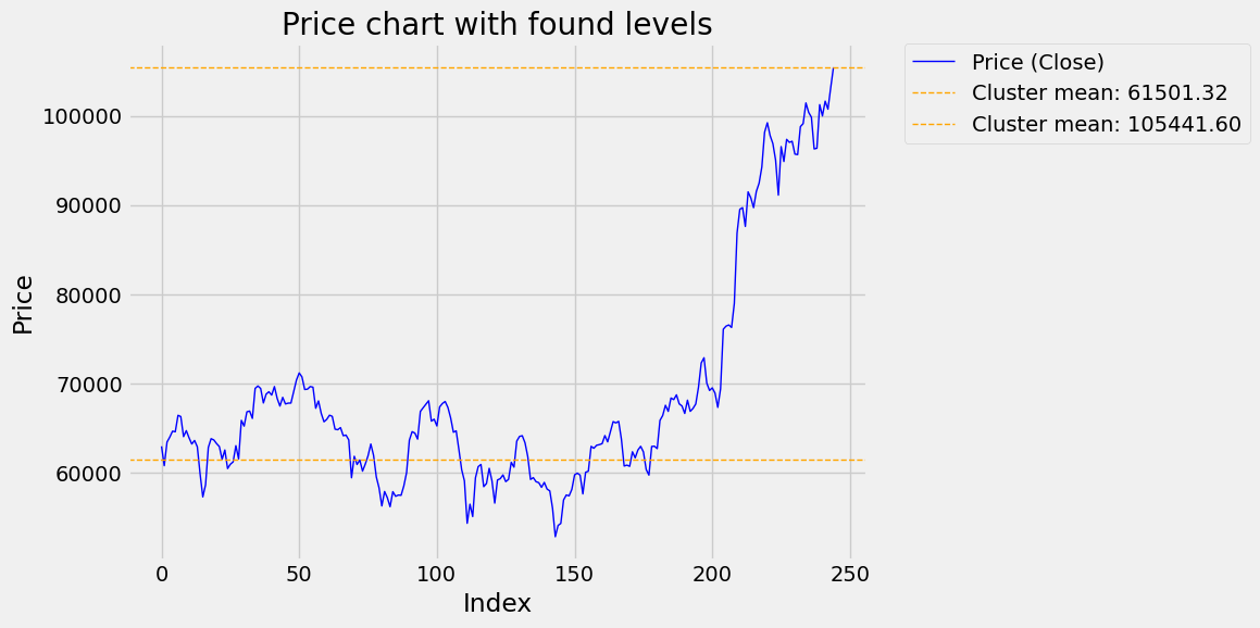
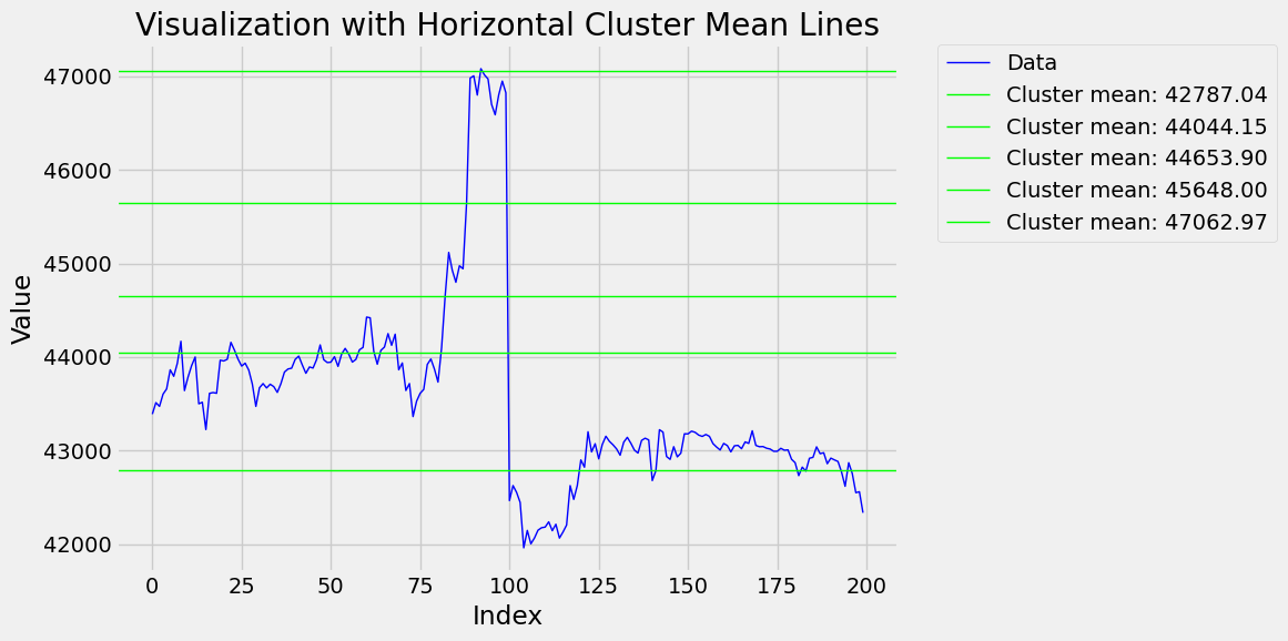
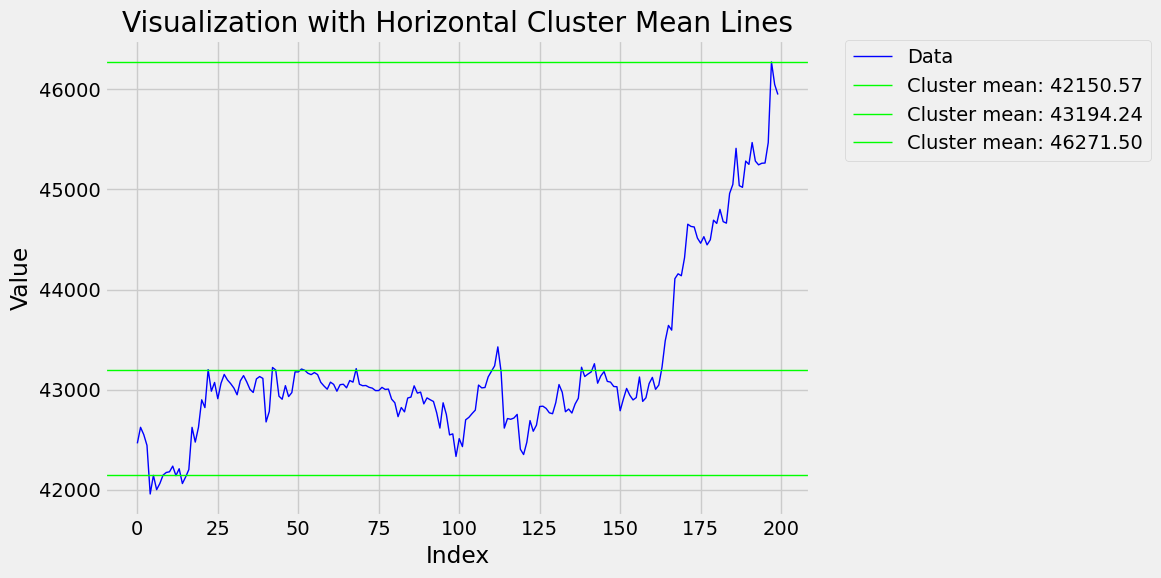
We will now attempt to segment the charts in various ways to evaluate the accuracy of the constructed levels.
1
2
3
4
5
6
7
8
9
10
11
12
13
14
15
16
17
18
19
20
21
22
23
24
25
26
27
28
29
30
31
32
33
34
35
def plot_with_clusters(data, cluster_means, width_line=1):
    """
    Visualizes the data with horizontal lines representing the mean values of clusters.

    Parameters:
    - data (np.ndarray): Array of data to be plotted.
    - cluster_means (list or np.ndarray): Mean values of the identified clusters.
    - width_line (float): Line width for cluster mean indicators (default is 1).
    """
    # Create the figure and axis
    fig, ax = plt.subplots(figsize=(12, 6))

    # Plot the data
    ax.plot(data, label='Data', color='blue', linewidth=1)

    # Add horizontal lines for each cluster mean
    for mean in cluster_means:
        ax.axhline(mean, color='lime', label=f'Cluster mean: {mean:.2f}', linewidth=width_line)

    # Configure plot appearance
    ax.set_title('Visualization with Horizontal Cluster Mean Lines')
    ax.set_xlabel('Index')
    ax.set_ylabel('Value')

    # Add a legend, avoiding duplicate labels
    handles, labels = ax.get_legend_handles_labels()
    by_label = dict(zip(labels, handles))
    ax.legend(by_label.values(), by_label.keys(), loc='upper left', bbox_to_anchor=(1.05, 1), borderaxespad=0.)

    # Enable grid
    ax.grid(True)

    # Display the plot
    plt.tight_layout()
    plt.show()
We will encapsulate the previously described code into a function for enhanced modularity.
1
2
3
4
5
6
7
8
9
10
11
12
13
14
15
16
17
18
19
20
21
22
23
24
25
26
27
28
29
30
31
32
33
34
35
36
37
38
39
40
41
42
43
44
45
46
47
48
49
50
51
52
def process_and_split_data(ext_price, all_close):
    """
    Processes data to compute new minimum and maximum values, shifts data,
    and segments arrays based on identified indices.

    Parameters:
    - ext_price (pd.DataFrame): DataFrame containing minimum, maximum values and indices.
    - all_close (np.ndarray): Data array to be segmented.

    Returns:
    tuple: A list of subarrays and an array of split indices.
    """
    # Shift the data by one row downward
    shifted_df = ext_price.shift()

    # Conditions: Minimum of the first row < Maximum of the second row
    condition1 = shifted_df['Maximum'] > ext_price['Minimum']
    condition2 = shifted_df['Minimum'] < ext_price['Maximum']

    # Compute new minimum and maximum values between current and next rows
    new_minimum = ext_price['Minimum'].combine(shifted_df['Minimum'], min).where(condition1)
    new_maximum = ext_price['Maximum'].combine(shifted_df['Maximum'], max)

    # Assign indices to new values
    new_min_index = ext_price['Min_Index'].where(new_minimum == ext_price['Minimum'], other=shifted_df['Min_Index'])
    new_max_index = ext_price['Max_Index'].where(new_maximum == ext_price['Maximum'], other=shifted_df['Max_Index'])

    # Form a new DataFrame with results
    result = pd.DataFrame({
        'New_Minimum': new_minimum,
        'New_Min_Index': new_min_index,
        'New_Maximum': new_maximum,
        'New_Max_Index': new_max_index
    })

    # Array to store segmentation indices
    splice_indices = np.empty(shape=0, dtype=int)
    for _, row in result.iterrows():
        if row['New_Min_Index'] > row['New_Max_Index']:
            new_values = np.array([row['New_Min_Index'], row['New_Max_Index']], dtype=int)
            splice_indices = np.append(splice_indices, new_values)

    # Sort and remove duplicate indices
    splice_indices = np.unique(splice_indices)

    # Exclude zero entries
    splice_indices = splice_indices[splice_indices != 0]

    # Segment the data array
    arrs = np.split(all_close, splice_indices)

    return arrs, splice_indices
Window analysis with varying slices
1
2
3
4
5
6
7
8
9
10
11
12
13
14
15
16
17
18
19
20
21
22
23
24
25
26
27
28
29
30
31
32
33
34
35
36
37
38
39
40
41
42
43
44
45
46
47
48
49
50
51
52
53
54
55
56
57
58
59
60
61
62
63
64
65
66
67
68
69
70
71
72
73
74
75
76
77
78
79
80
81
82
83
84
85
86
87
88
89
90
# Define the range for window sizes
min_length = 100
max_length = len(df)
step = 100
window_size = 200  # Window size

# List to store results
final_results = []

# Loop through different slices
for start in range(min_length, max_length - window_size + 1, step):
    end = start + window_size
    slice_candles = df.iloc[start:end]  # Extract slice

    # Ensure the slice is not empty
    if slice_candles.empty:
        print(f"Empty slice: start={start}, end={end}, skipping iteration.")
        continue

    # Example processing for the current slice
    all_close = slice_candles['Close'].values
    all_close = all_close[~np.isnan(all_close)]  # Remove NaN values

    divider = len(all_close) // 20  # Block size
    shift_increment = 5  # Increment for shifts
    max_shift = len(all_close) // 2  # Maximum shift

    rows = []

    for shift in range(20, max_shift, shift_increment):
        # Use `process_extreme_values` and `find_extr` functions
        result_df, splice_indices = process_extreme_values(find_extr(all_close, divider, shift))

        arrs = np.split(all_close, splice_indices)
        for i, subarray in enumerate(arrs):
            if subarray.size == 0:
                continue

            min_value = np.min(subarray)
            max_value = np.max(subarray)

            rows.append({
                'Shift': shift,
                'Array': i + 1,
                'Min': min_value,
                'Max': max_value
            })

    arr_count = pd.DataFrame(rows)
    grouped = arr_count.groupby(['Array', 'Min', 'Max'])
    result = grouped['Shift'].nunique().reset_index(name='Shift_Count')
    matches = result[result['Shift_Count'] > 1].copy()

    all_values = np.concatenate([matches['Min'].values, matches['Max'].values])
    std_dev = np.std(all_values)
    mean_value = np.mean(all_values)
    threshold = 0.3 * std_dev

    sorted_values = np.sort(all_values)
    clusters = []
    current_cluster = []

    for value in sorted_values:
        if not current_cluster:
            current_cluster.append(value)
        else:
            if value - current_cluster[-1] <= threshold:
                current_cluster.append(value)
            else:
                clusters.append(current_cluster)
                current_cluster = [value]

    if current_cluster:
        clusters.append(current_cluster)

    cluster_means = [np.mean(cluster) for cluster in clusters]

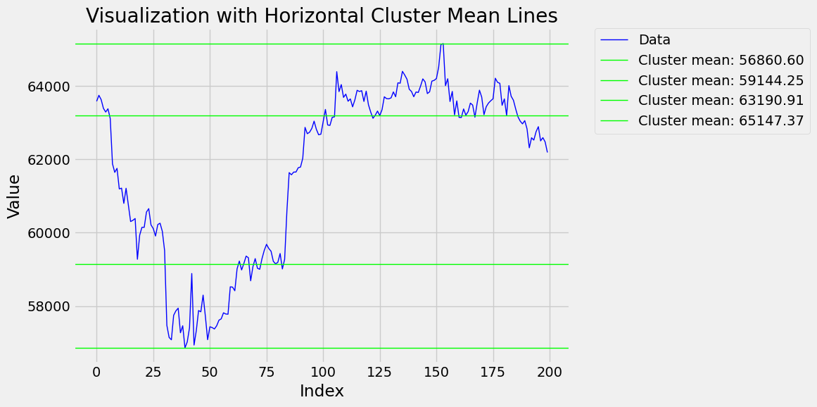
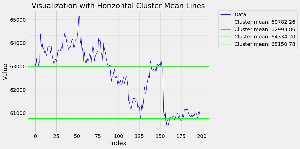
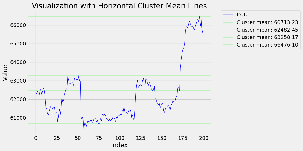
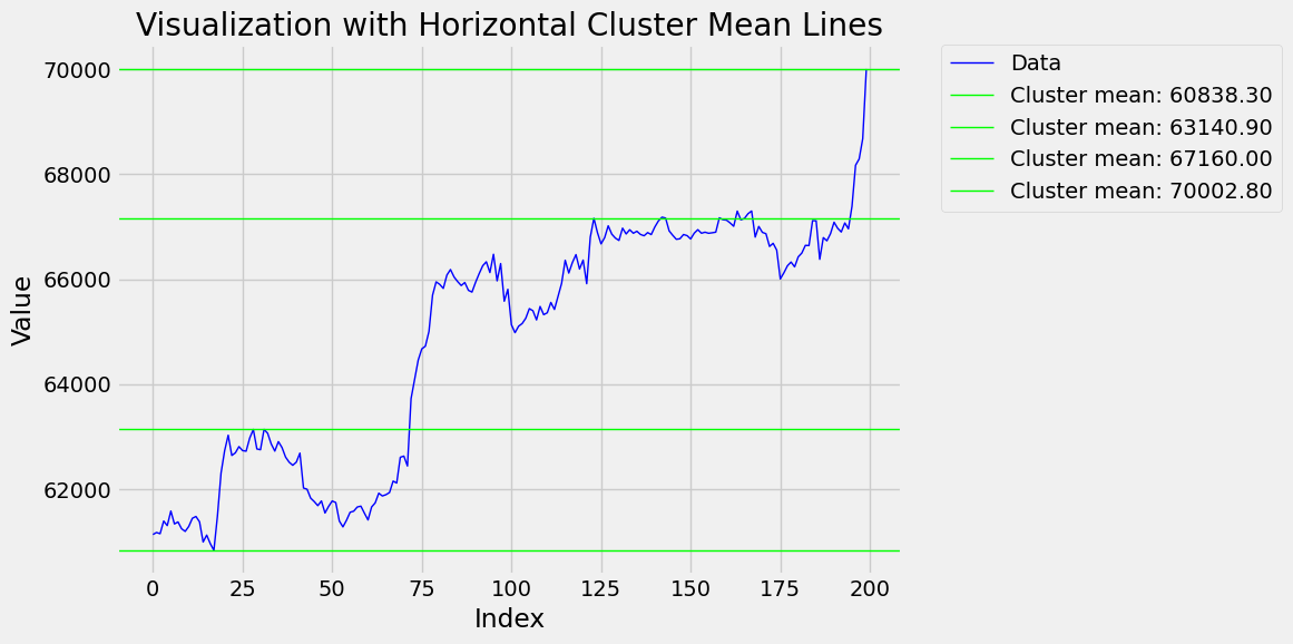
    plot_with_clusters(all_close, cluster_means, width_line=1)

    # Store results for the current slice
    final_results.append({
        'Window_Start': start,
        'Window_End': end,
        'Cluster_Means': cluster_means
    })

# Output results
for result in final_results:
    print(f"Slice: {result['Window_Start']}:{result['Window_End']}, Cluster Means: {result['Cluster_Means']}")
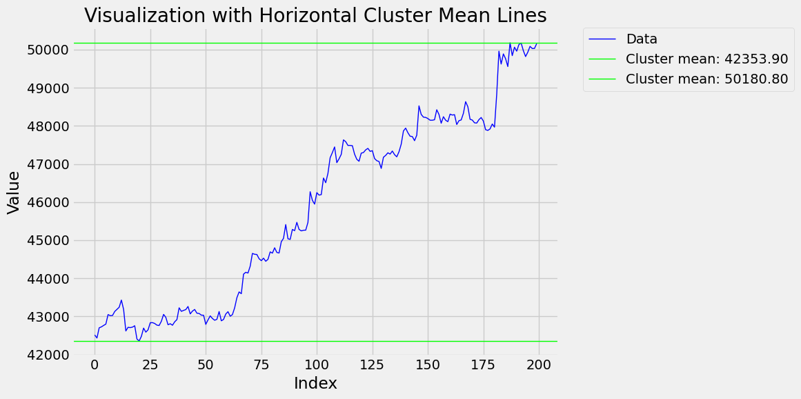
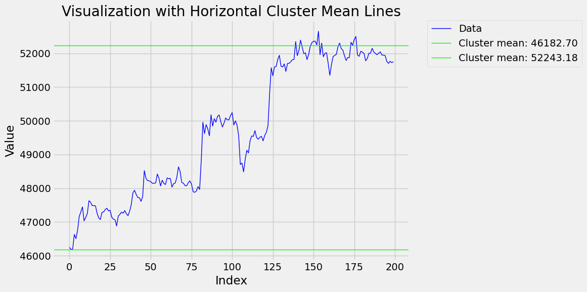
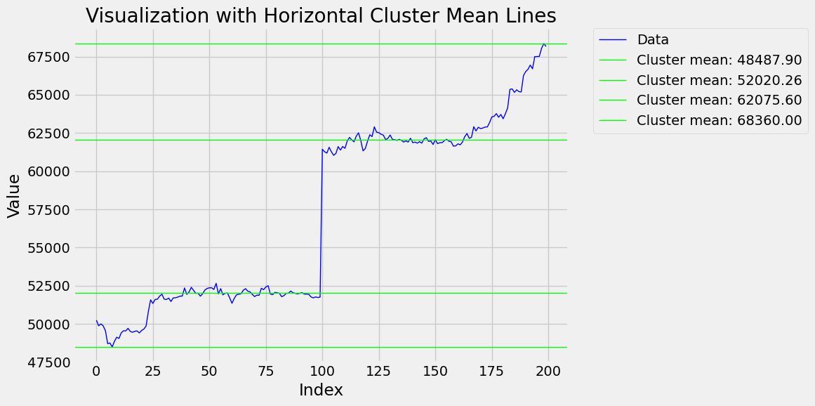
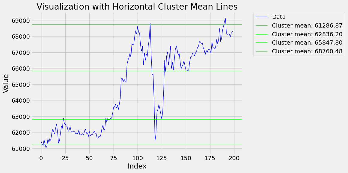
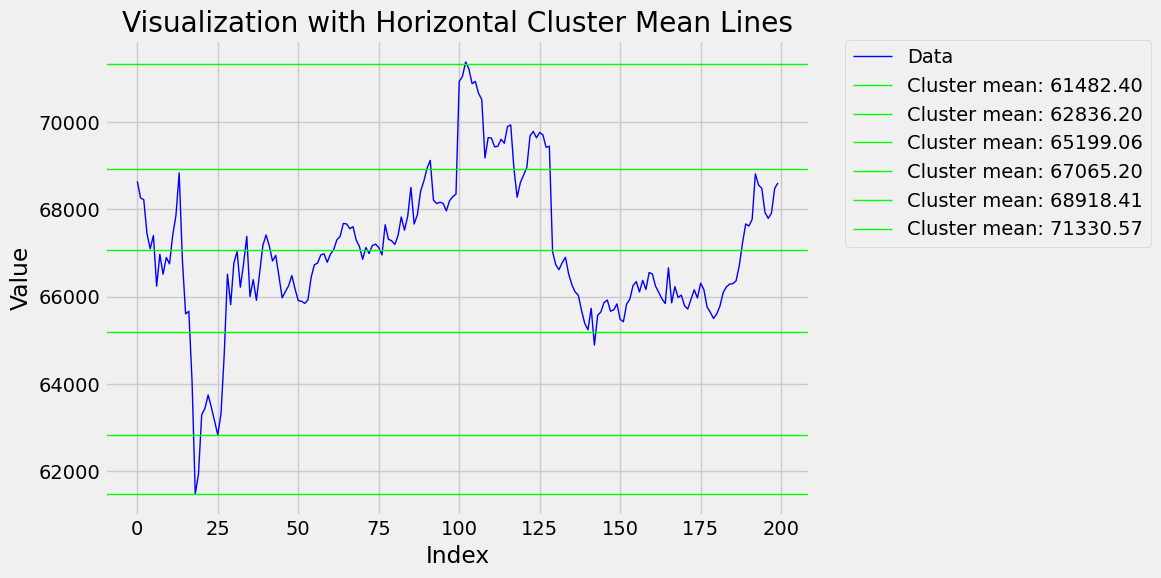
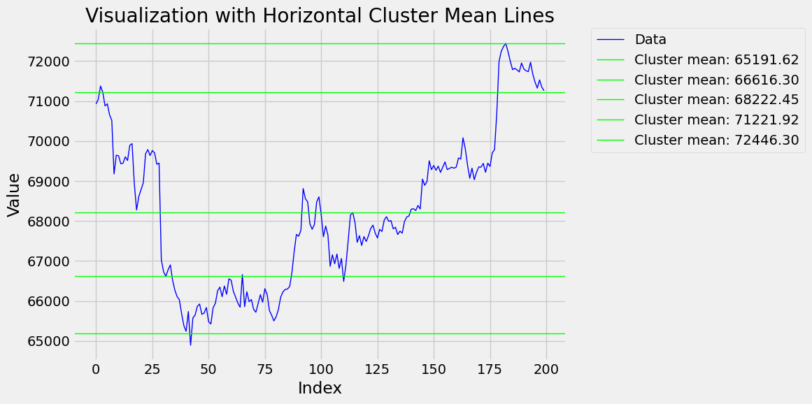
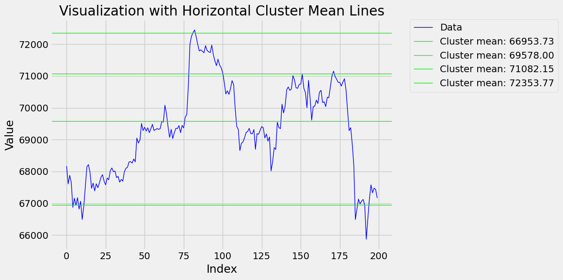
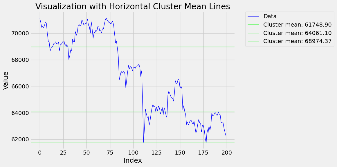
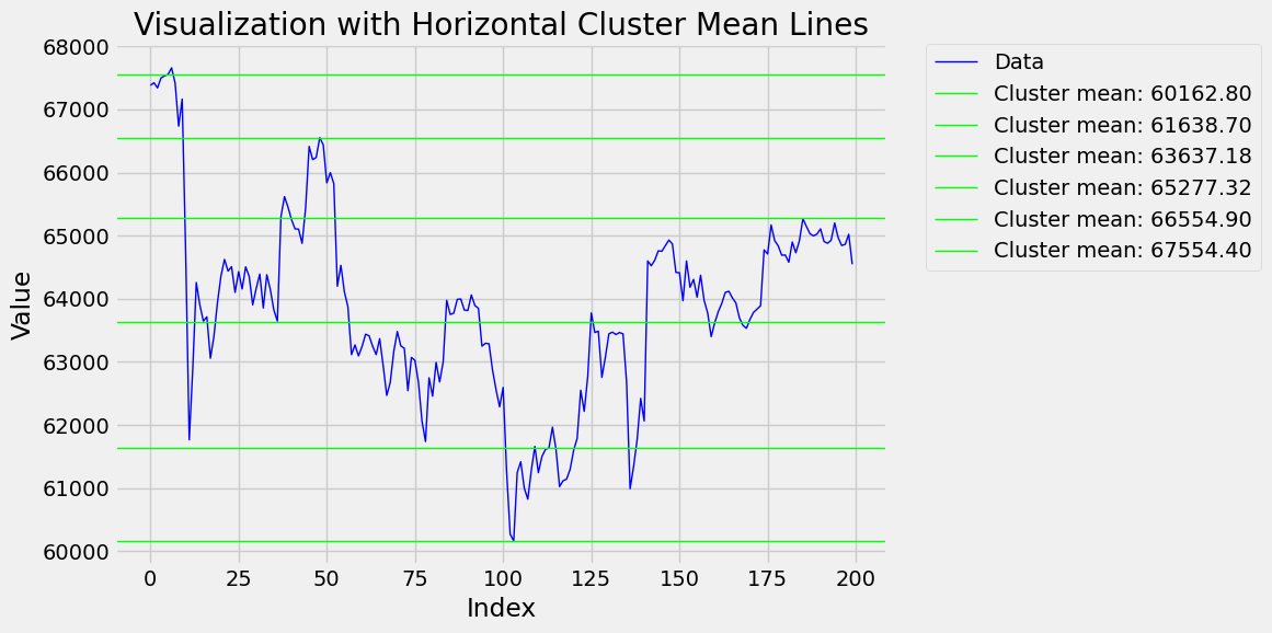
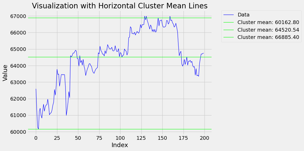
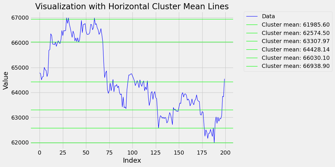
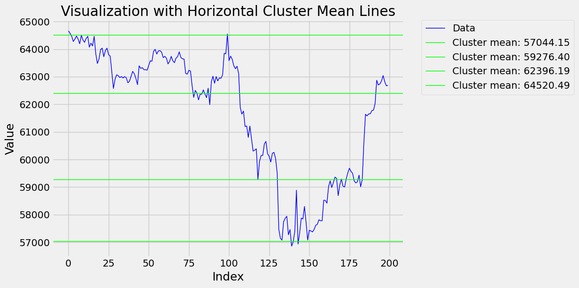
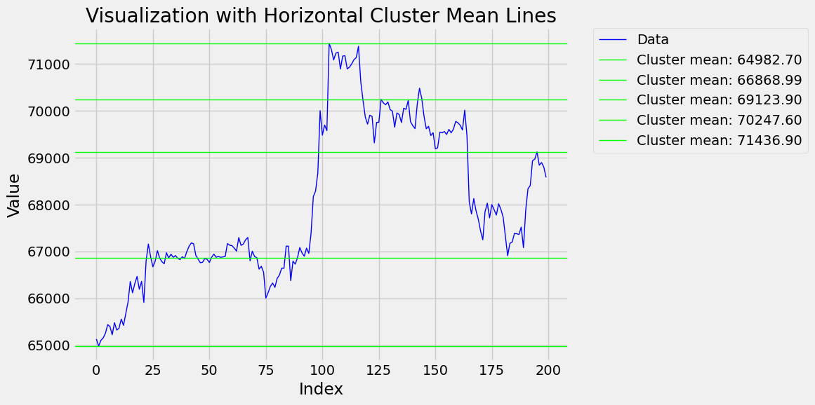
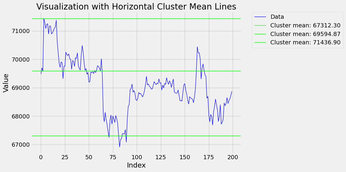
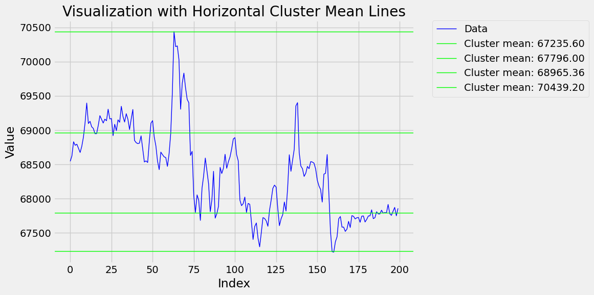
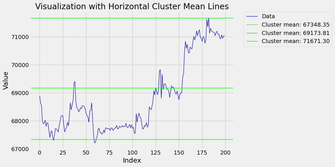
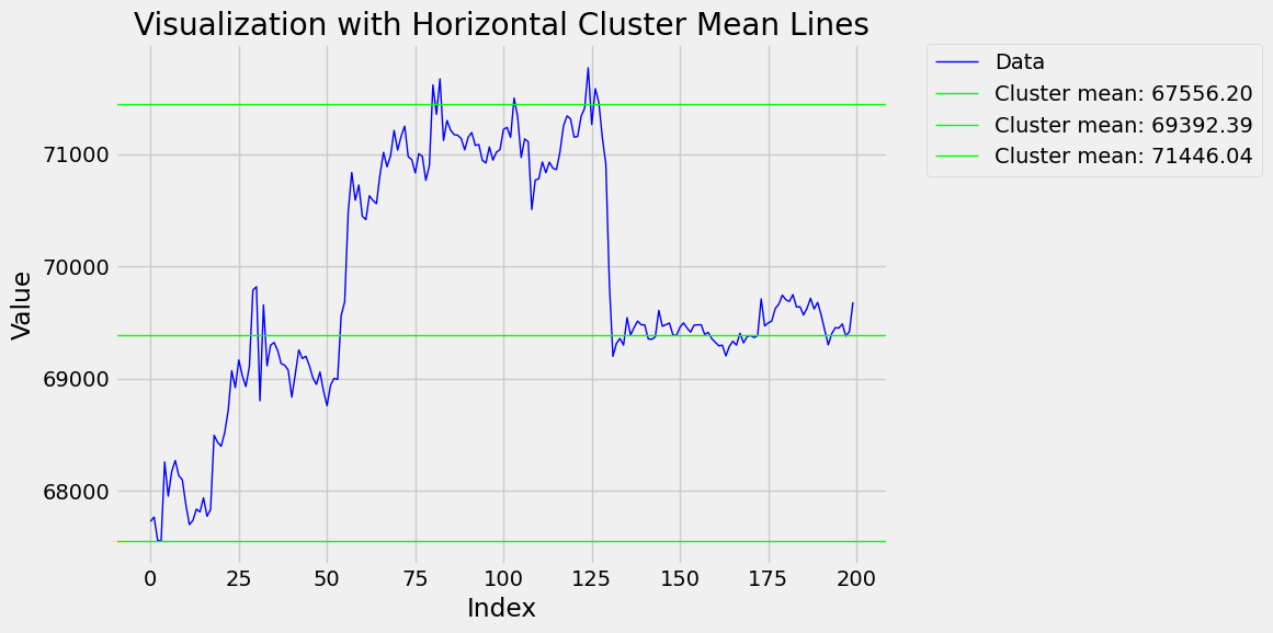
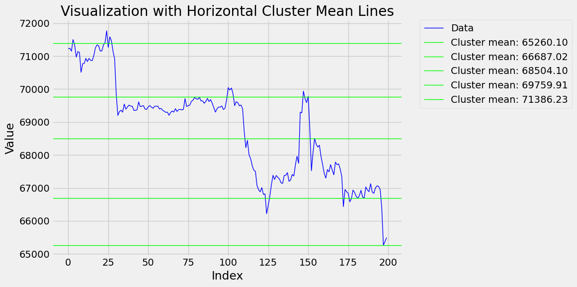
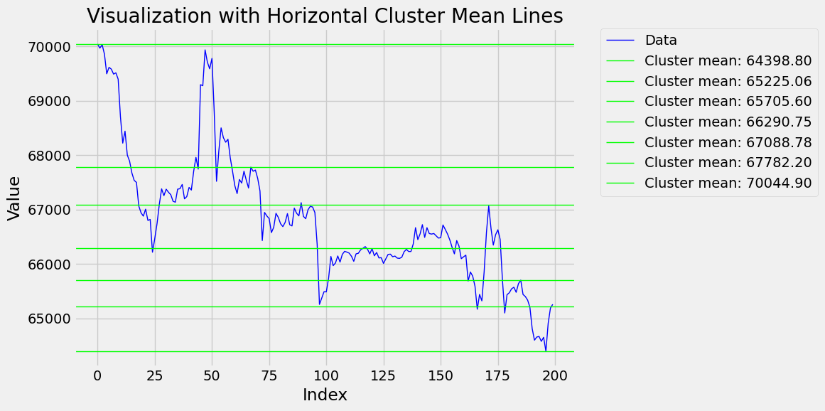
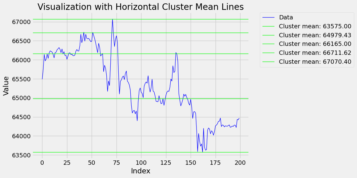
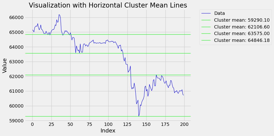
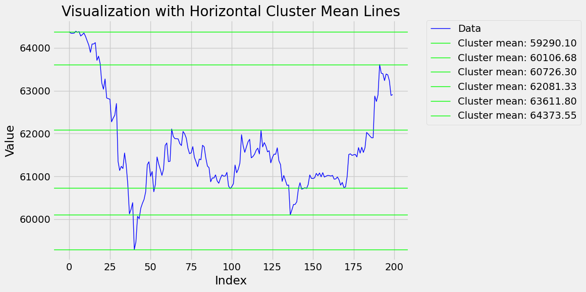
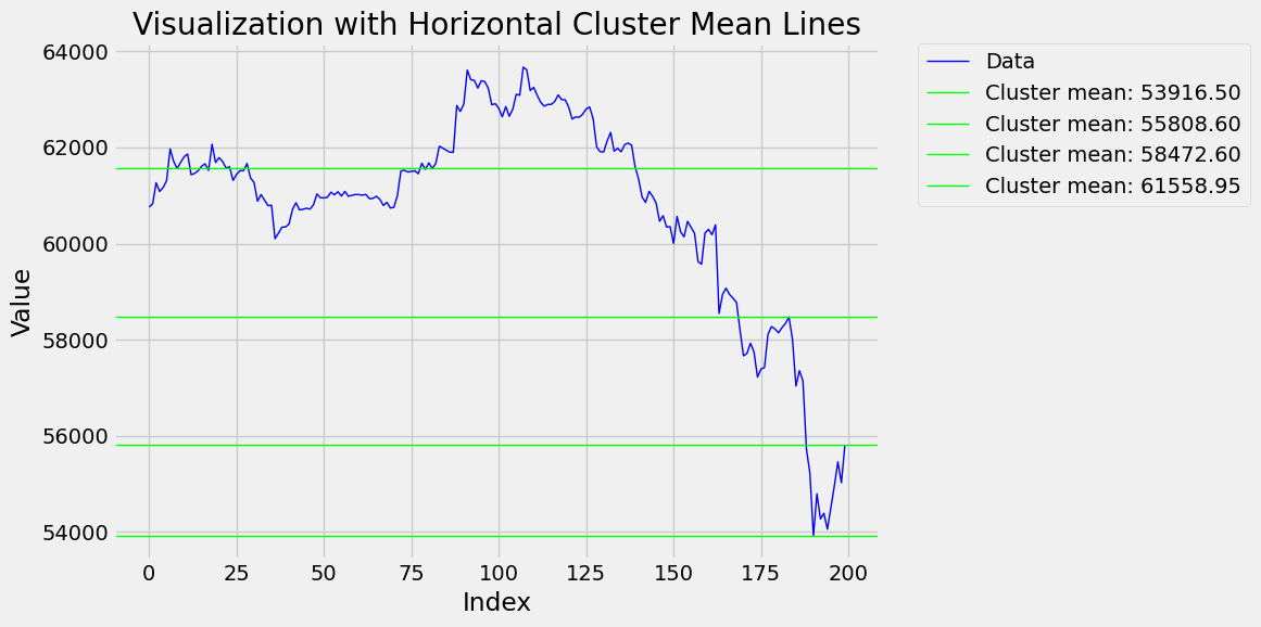
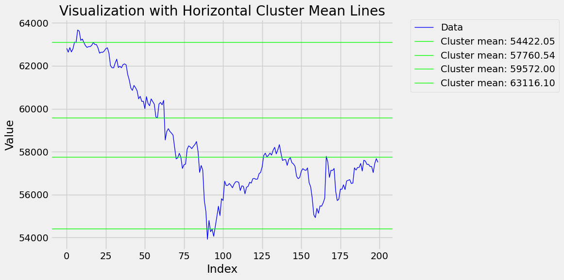
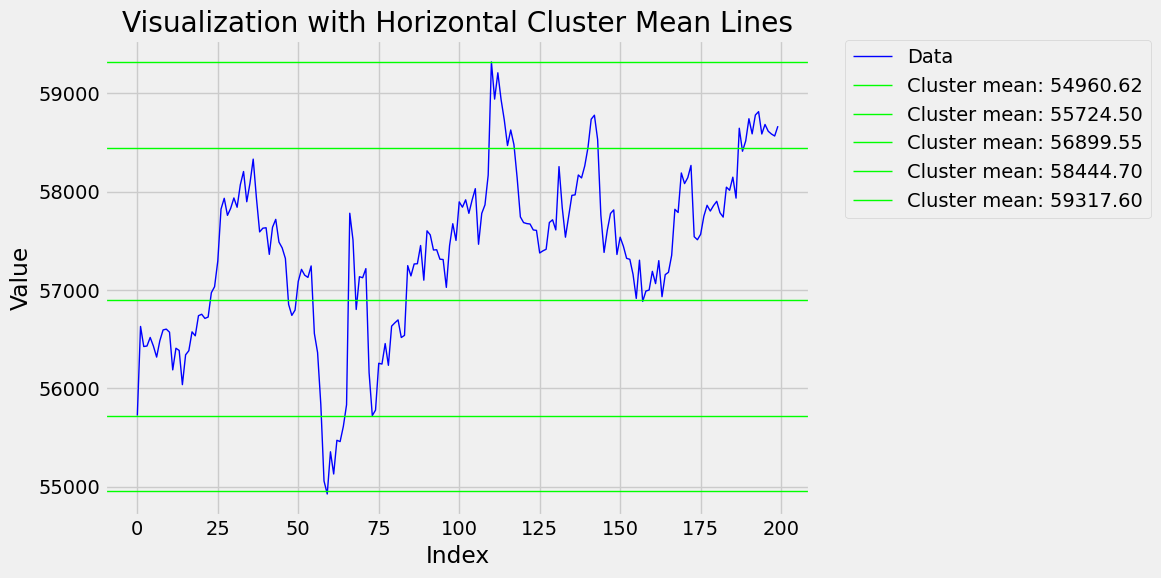
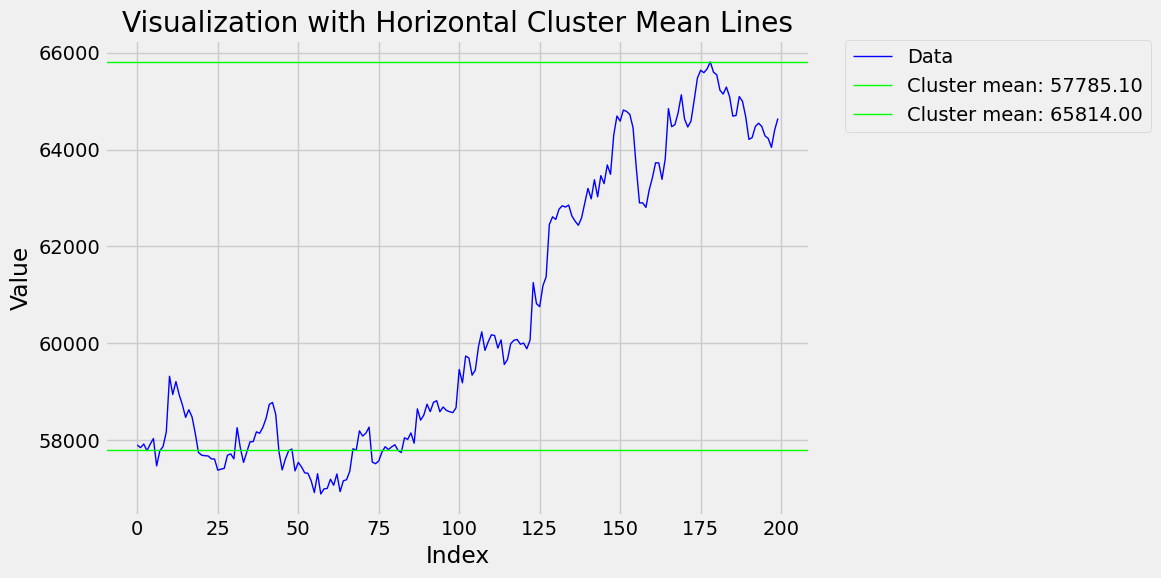
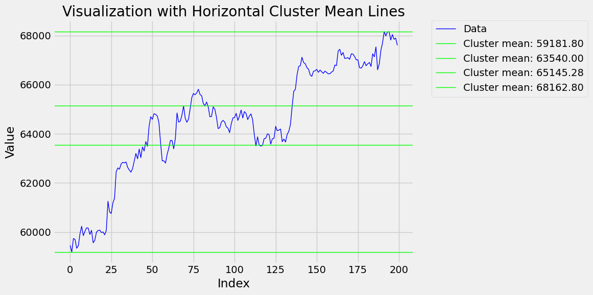
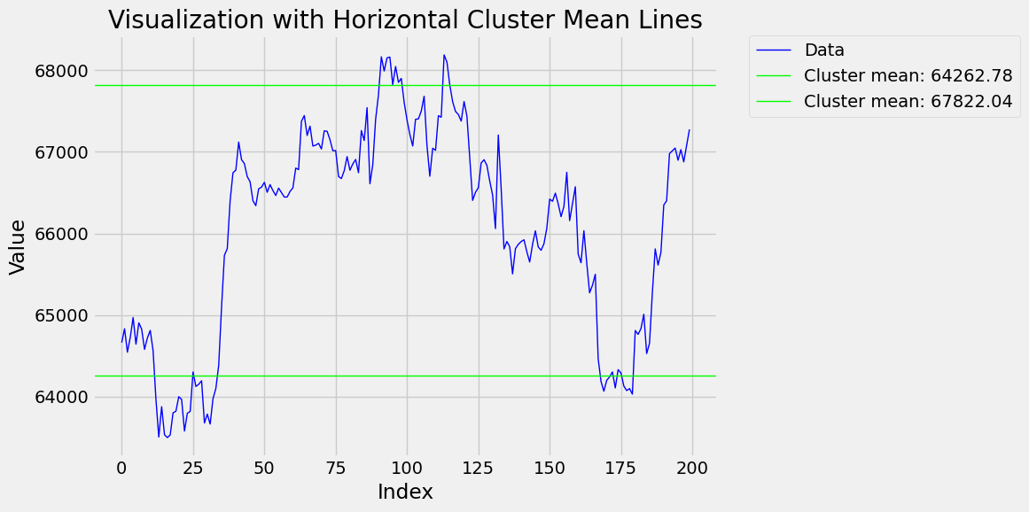
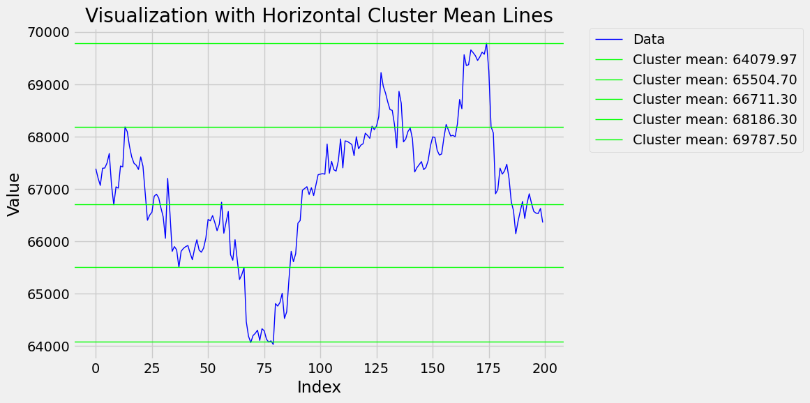
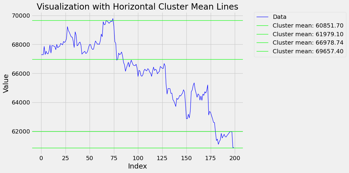
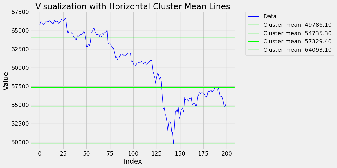
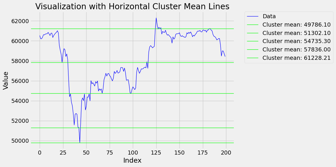
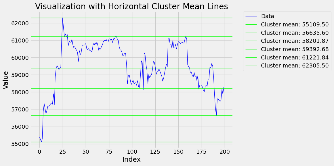
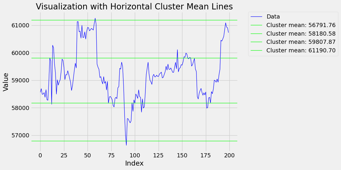
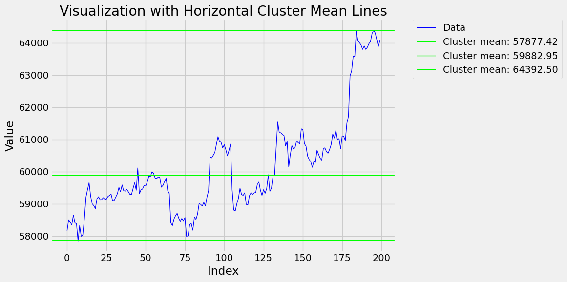
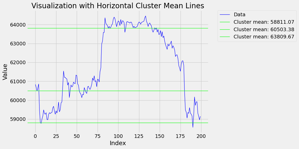
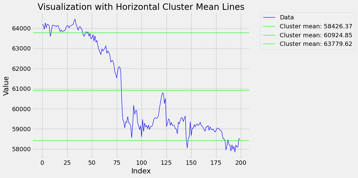
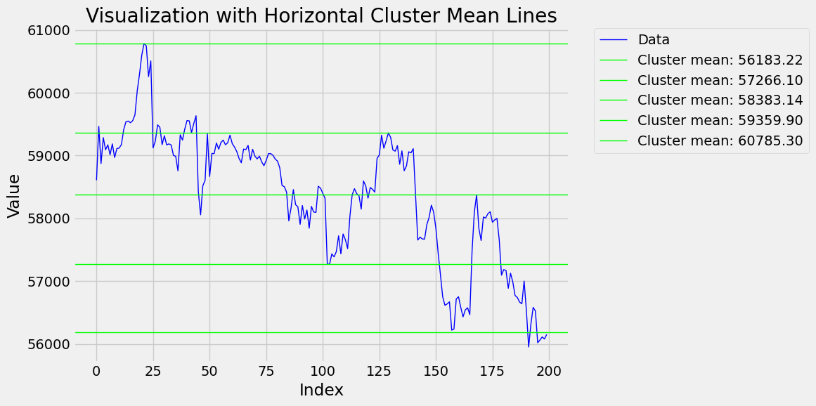
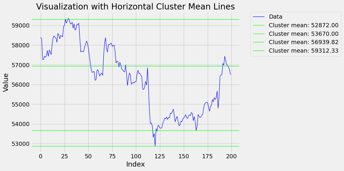
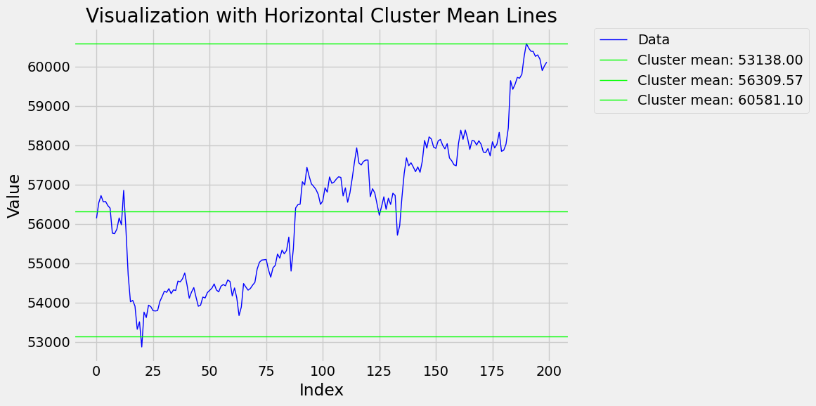
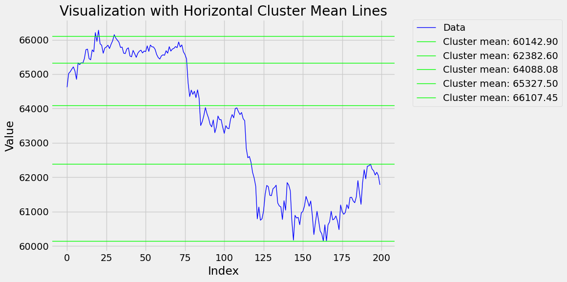
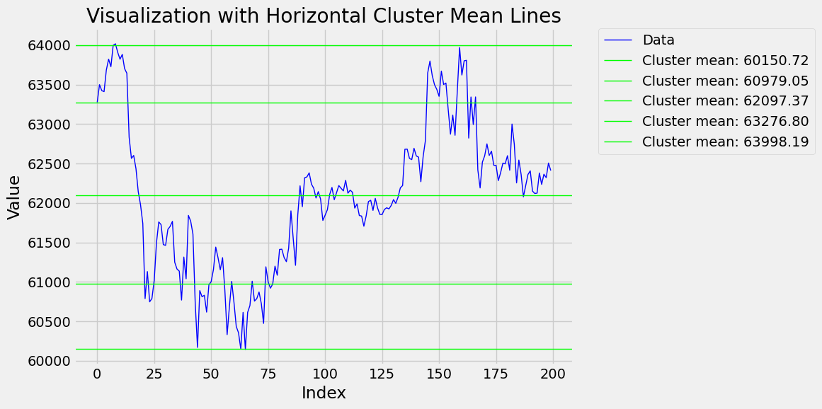
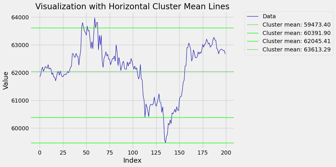
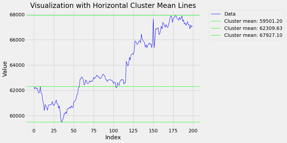
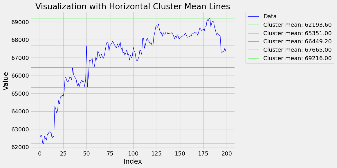
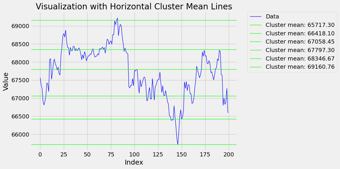
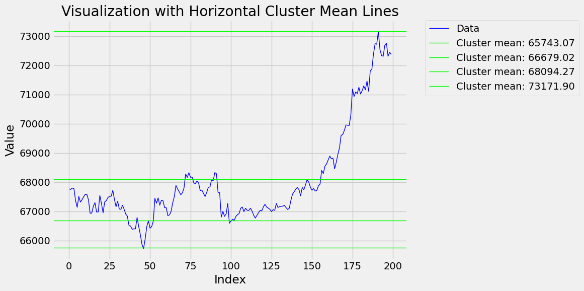
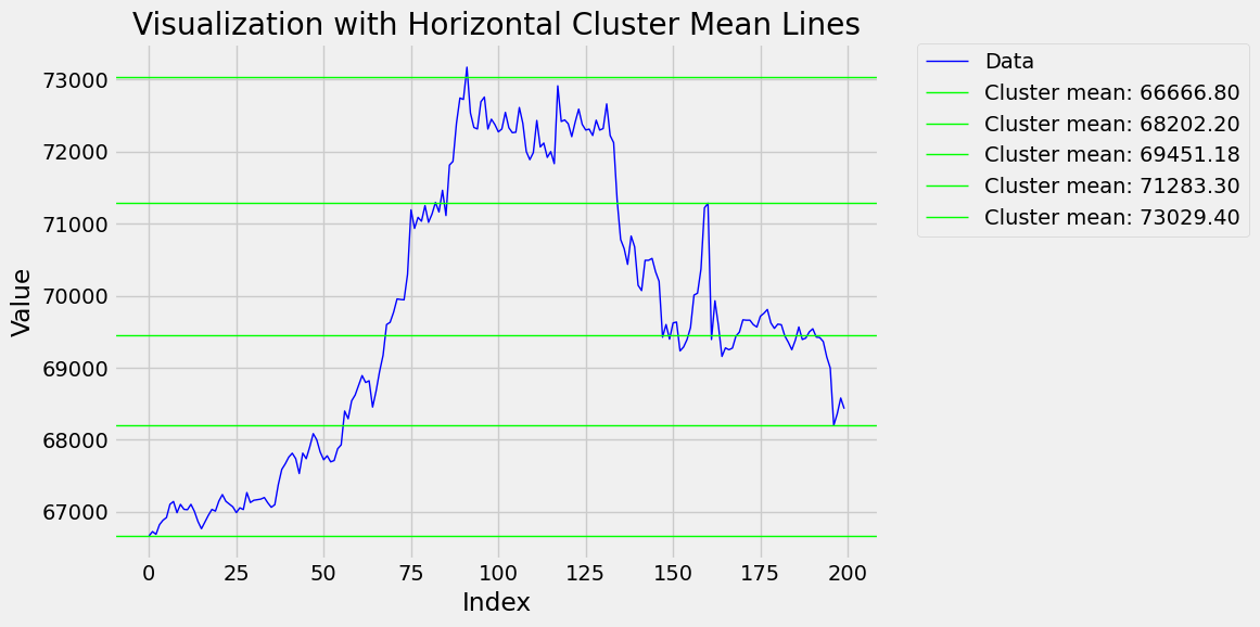
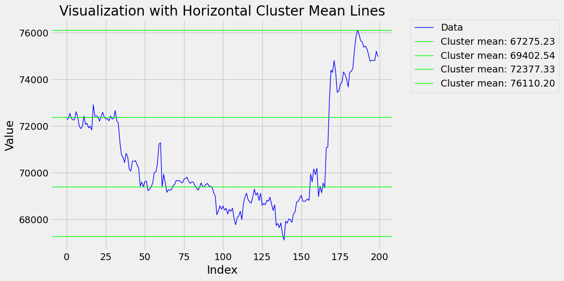
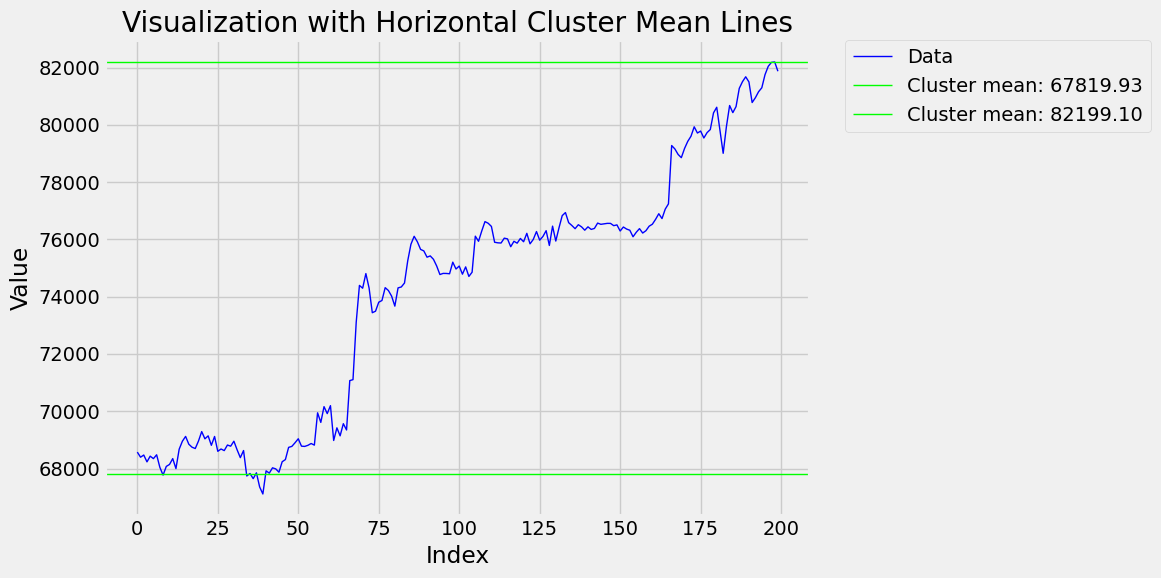
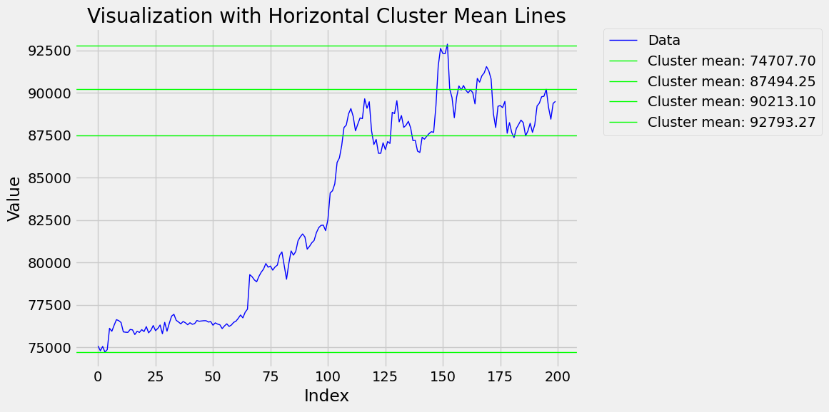
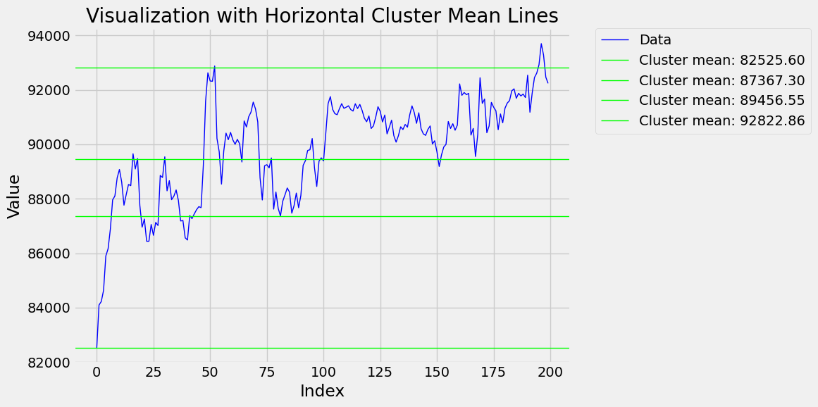
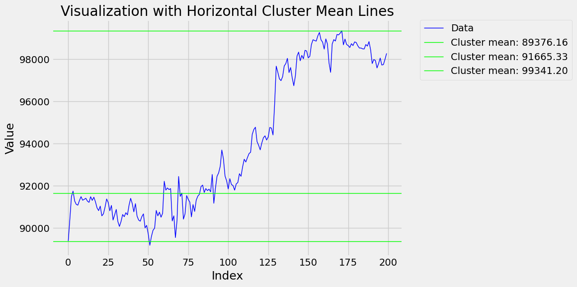
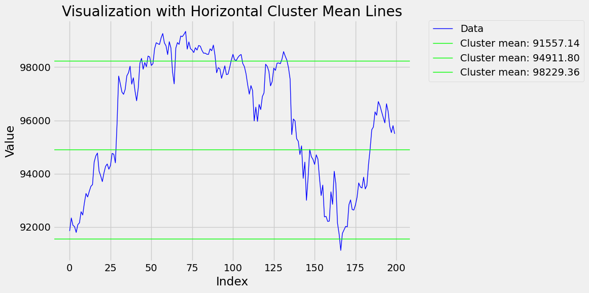
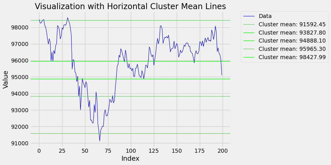
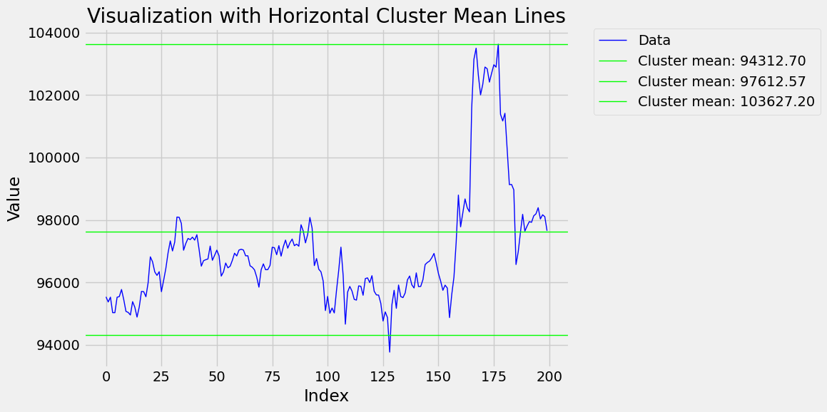
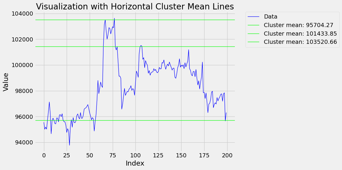
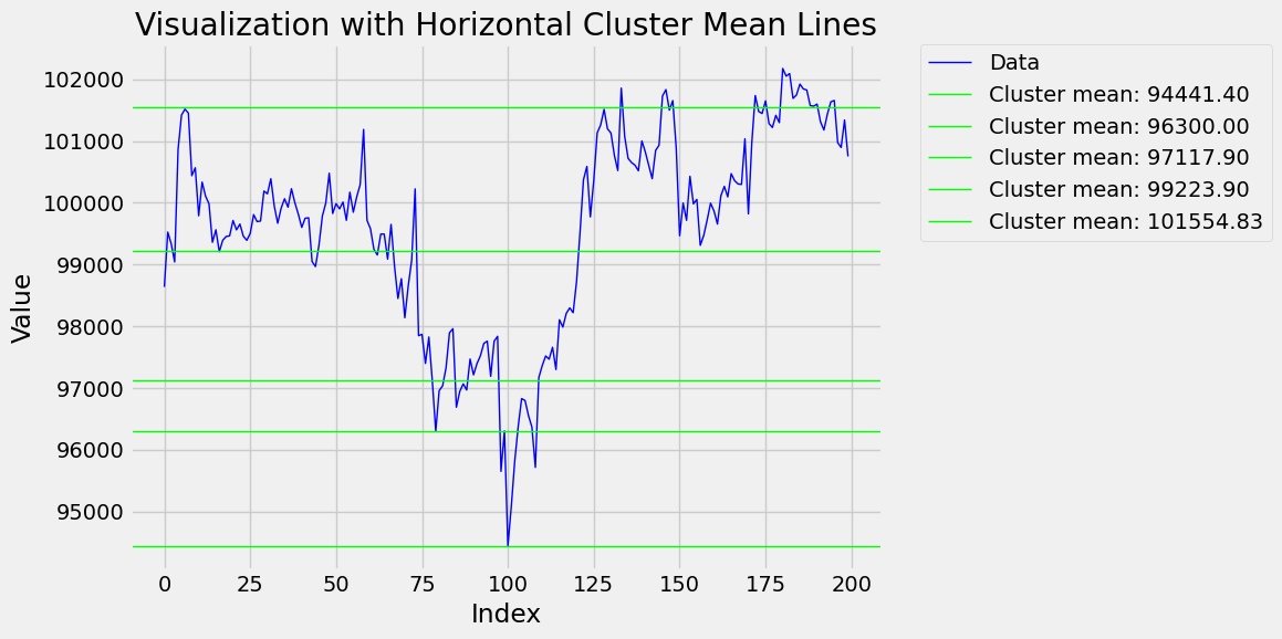
1
2
3
4
5
6
7
8
9
10
11
12
13
14
15
16
17
18
19
20
21
22
23
24
25
26
27
28
29
30
31
32
33
34
35
36
37
38
39
40
41
42
43
44
45
46
47
48
49
50
51
52
53
54
55
56
57
58
59
60
61
62
63
64
65
66
67
68
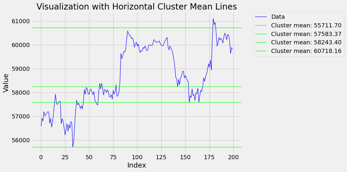
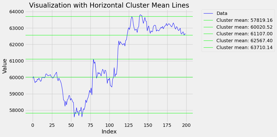
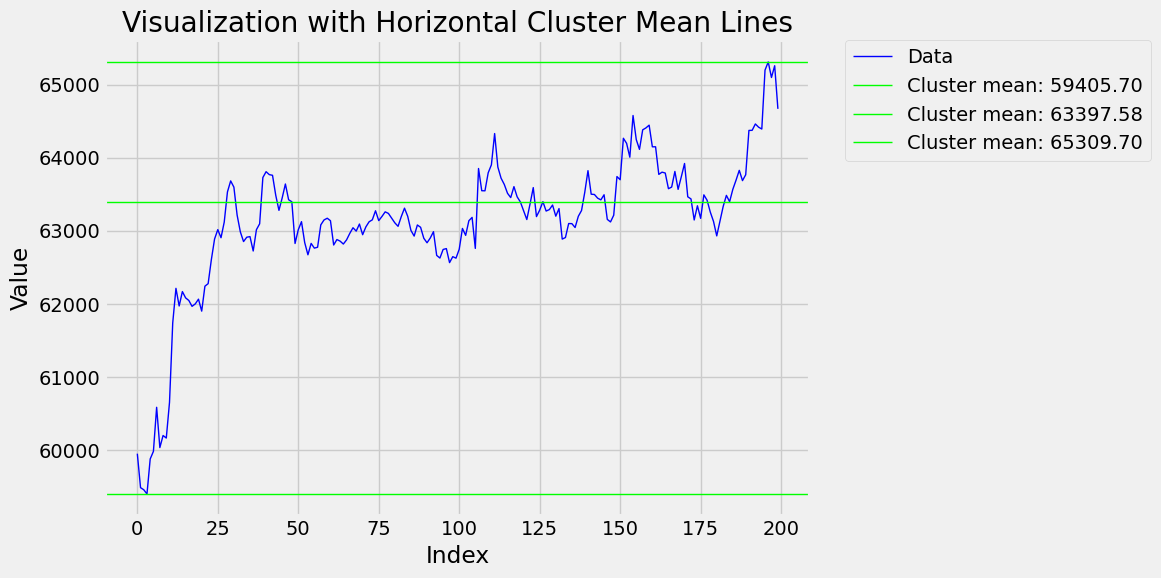
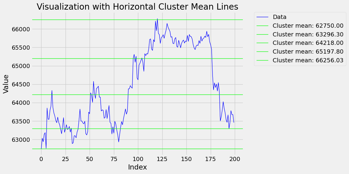
Slice: 100:300, Cluster Means: [42787.045, 44044.15, 44653.9, 45648.0, 47062.975]
Slice: 200:400, Cluster Means: [42150.566666666666, 43194.24, 46271.5]
Slice: 300:500, Cluster Means: [42353.9, 50180.8]
Slice: 400:600, Cluster Means: [46182.7, 52243.18333333333]
Slice: 500:700, Cluster Means: [48487.9, 52020.2625, 62075.6, 68360.0]
Slice: 600:800, Cluster Means: [61286.86666666667, 62836.2, 65847.8, 68760.475]
Slice: 700:900, Cluster Means: [61482.4, 62836.2, 65199.0625, 67065.20000000001, 68918.41, 71330.57142857143]
Slice: 800:1000, Cluster Means: [65191.62000000001, 66616.3, 68222.45, 71221.92, 72446.3]
Slice: 900:1100, Cluster Means: [66953.73333333334, 69578.0, 71082.15, 72353.76666666666]
Slice: 1000:1200, Cluster Means: [61748.9, 64061.1, 68974.37333333335]
Slice: 1100:1300, Cluster Means: [60162.8, 61638.7, 63637.18000000001, 65277.325, 66554.9, 67554.4]
Slice: 1200:1400, Cluster Means: [60162.8, 64520.544444444444, 66885.4]
Slice: 1300:1500, Cluster Means: [61985.6, 62574.5, 63307.975, 64428.1375, 66030.1, 66938.9]
Slice: 1400:1600, Cluster Means: [57044.15, 59276.4, 62396.185714285704, 64520.4875]
Slice: 1500:1700, Cluster Means: [56860.6, 59144.25, 63190.912500000006, 65147.36666666667]
Slice: 1600:1800, Cluster Means: [60782.261538461535, 62993.86470588236, 64334.200000000004, 65150.780000000006]
Slice: 1700:1900, Cluster Means: [60713.225000000006, 62482.450000000004, 63258.166666666664, 66476.1]
Slice: 1800:2000, Cluster Means: [60838.30000000001, 63140.9, 67160.0, 70002.8]
Slice: 1900:2100, Cluster Means: [64982.7, 66868.9909090909, 69123.9, 70247.6, 71436.9]
Slice: 2000:2200, Cluster Means: [67312.3, 69594.8705882353, 71436.90000000001]
Slice: 2100:2300, Cluster Means: [67235.6, 67796.0, 68965.36249999999, 70439.2]
Slice: 2200:2400, Cluster Means: [67348.34615384614, 69173.8125, 71671.3]
Slice: 2300:2500, Cluster Means: [67556.2, 69392.38888888889, 71446.04]
Slice: 2400:2600, Cluster Means: [65260.1, 66687.025, 68504.1, 69759.91111111111, 71386.23333333334]
Slice: 2500:2700, Cluster Means: [64398.8, 65225.05714285715, 65705.6, 66290.75, 67088.78333333333, 67782.2, 70044.9]
Slice: 2600:2800, Cluster Means: [63575.0, 64979.42500000001, 66165.0, 66711.625, 67070.4]
Slice: 2700:2900, Cluster Means: [59290.1, 62106.6, 63575.0, 64846.18235294117]
Slice: 2800:3000, Cluster Means: [59290.1, 60106.675, 60726.3, 62081.333333333336, 63611.80000000001, 64373.55]
Slice: 2900:3100, Cluster Means: [53916.5, 55808.6, 58472.6, 61558.952631578955]
Slice: 3000:3200, Cluster Means: [54422.05, 57760.54285714286, 59572.0, 63116.100000000006]
Slice: 3100:3300, Cluster Means: [54960.625, 55724.5, 56899.55, 58444.7, 59317.6]
Slice: 3200:3400, Cluster Means: [57785.1, 65814.0]
Slice: 3300:3500, Cluster Means: [59181.80000000001, 63540.0, 65145.280000000006, 68162.8]
Slice: 3400:3600, Cluster Means: [64262.784615384604, 67822.03636363638]
Slice: 3500:3700, Cluster Means: [64079.975, 65504.7, 66711.3, 68186.3, 69787.5]
Slice: 3600:3800, Cluster Means: [60851.7, 61979.1, 66978.7388888889, 69657.4]
Slice: 3700:3900, Cluster Means: [49786.1, 54735.3, 57329.4, 64093.09999999999]
Slice: 3800:4000, Cluster Means: [49786.1, 51302.1, 54735.3, 57836.0, 61228.21428571428]
Slice: 3900:4100, Cluster Means: [55109.5, 56635.6, 58201.87142857142, 59392.675, 61221.840000000004, 62305.5]
Slice: 4000:4200, Cluster Means: [56791.759999999995, 58180.57777777778, 59807.86666666667, 61190.69999999999]
Slice: 4100:4300, Cluster Means: [57877.424999999996, 59882.95, 64392.5]
Slice: 4200:4400, Cluster Means: [58811.06999999999, 60503.380000000005, 63809.66666666666]
Slice: 4300:4500, Cluster Means: [58426.372727272734, 60924.85, 63779.62105263159]
Slice: 4400:4600, Cluster Means: [56183.225, 57266.1, 58383.142857142855, 59359.9, 60785.3]
Slice: 4500:4700, Cluster Means: [52872.0, 53670.0, 56939.82380952381, 59312.333333333336]
Slice: 4600:4800, Cluster Means: [53138.0, 56309.575, 60581.1]
Slice: 4700:4900, Cluster Means: [55711.7, 57583.37499999999, 58243.4, 60718.15555555556]
Slice: 4800:5000, Cluster Means: [57819.15714285715, 60020.524999999994, 61107.0, 62567.4, 63710.14]
Slice: 4900:5100, Cluster Means: [59405.69999999999, 63397.57777777777, 65309.7]
Slice: 5000:5200, Cluster Means: [62750.0, 63296.3, 64218.0, 65197.8, 66256.03333333334]
Slice: 5100:5300, Cluster Means: [60142.9, 62382.6, 64088.08, 65327.5, 66107.45]
Slice: 5200:5400, Cluster Means: [60150.725, 60979.05, 62097.36666666667, 63276.8, 63998.1875]
Slice: 5300:5500, Cluster Means: [59473.4, 60391.9, 62045.41428571429, 63613.2875]
Slice: 5400:5600, Cluster Means: [59501.200000000004, 62309.63333333334, 67927.1]
Slice: 5500:5700, Cluster Means: [62193.6, 65351.0, 66449.2, 67665.0, 69216.0]
Slice: 5600:5800, Cluster Means: [65717.3, 66418.1, 67058.45000000001, 67797.3, 68346.66666666667, 69160.75714285714]
Slice: 5700:5900, Cluster Means: [65743.06666666667, 66679.02222222224, 68094.27499999998, 73171.9]
Slice: 5800:6000, Cluster Means: [66666.8, 68202.2, 69451.18000000001, 71283.3, 73029.4]
Slice: 5900:6100, Cluster Means: [67275.225, 69402.54285714285, 72377.32999999999, 76110.2]
Slice: 6000:6200, Cluster Means: [67819.925, 82199.1]
Slice: 6100:6300, Cluster Means: [74707.7, 87494.25, 90213.1, 92793.26666666666]
Slice: 6200:6400, Cluster Means: [82525.6, 87367.3, 89456.54999999999, 92822.85714285714]
Slice: 6300:6500, Cluster Means: [89376.16, 91665.33333333333, 99341.2]
Slice: 6400:6600, Cluster Means: [91557.14444444445, 94911.8, 98229.35625]
Slice: 6500:6700, Cluster Means: [91592.45, 93827.8, 94888.1, 95965.3, 98427.98571428572]
Slice: 6600:6800, Cluster Means: [94312.70000000001, 97612.56666666665, 103627.2]
Slice: 6700:6900, Cluster Means: [95704.27142857143, 101433.85, 103520.65714285713]
Slice: 6800:7000, Cluster Means: [94441.4, 96300.0, 97117.9, 99223.9, 101554.83333333333]
This code performs the following actions:
Defines a range of window sizes for data analysis.
Creates an empty list to store the results of.
Passes through various data slices, starting with the minimum size and ending with the maximum size, with the step specified in the step parameter.
For each data slice, retrieves data for the specified period.
Checks whether the slice is empty and skips the iteration if it is.
Performs an example of data processing for the current slice.
Creates a list for storing data processing results.
Runs through various shift values to find extreme values of.
Creates a DataFrame with the results of data processing for each shift.
Groups data into three columns and finds unique values for each shift.
Selects only those shifts for which the number of unique values is greater than 1.
Creates an array with all the minimum and maximum values of found.
Calculates the standard deviation and average value for the array.
Finds a threshold for determining clusters based on the standard deviation.
Sorts an array with values.
Creates clusters based on sorted values and the threshold.
Calculates the average value for each cluster.
Builds a graph with clusters and source data.
Saves the results of data processing for the current slice in the final_results list.
Displays the results of data processing for each slice.
Code Comments:
At the beginning of the code, parameters for data analysis are defined, such as the window size range, step, and shift size.
For each data slice, data is processed and the results are stored in the final_results list.
The code uses various functions for data processing, such as finding extreme values, creating clusters, and plotting.
The results of data processing are displayed on the screen for each slice.
6. Conclusion
The analysis demonstrated the feasibility of identifying significant support and resistance levels using algorithmic techniques. However, further work is required to refine the algorithms, particularly for handling high market volatility and optimizing computational efficiency. Future studies could explore alternative methods such as machine learning models or volume profile analysis to enhance the accuracy of level identification. Real-time application and validation of these techniques remain a promising area for development.
7. Comprehensive understanding
I am sure that this work can be useful for readers, providing them with an alternative view of technical analysis and trading. These approaches will help novice traders better understand the basics of market data analysis and form their own vision of the market. However, it is important to remember that financial markets remain a high-risk environment, where methods such as those described do not guarantee success and require careful risk assessment.
This work inspired me to further study the data and develop new algorithms for analyzing noise levels. I see great potential for improving the proposed approach and adapting it to different market scenarios.